---
title: "Chapter 12: Non-Stationarity and Unit Roots"
subtitle: "Stationarity, spurious regression, ADF tests, and cointegration"
---
```{r}
#| label: setup
#| include: false
library(tidyverse)
library(broom)
library(modelsummary)
library(lmtest)
library(tseries)
library(dynlm)
library(wooldridge)
theme_set(theme_minimal(base_size = 13))
options(digits = 4, scipen = 999)
data("intdef", package = "wooldridge")
data("fertil3", package = "wooldridge")
data("phillips", package = "wooldridge")
set.seed(2024)
```
::: {.callout-note}
## Learning Objectives
By the end of this chapter you will be able to:
- Distinguish strict stationarity from weak (covariance) stationarity
- Derive the mean, variance, and autocorrelation of a random walk as functions of $t$
- Explain why the random walk violates all three stationarity conditions
- Derive the Dickey-Fuller (DF) test regression from the AR(1) model by algebraic subtraction
- State the three DF model variants (no constant, constant, constant + trend)
- Explain why DF/ADF critical values are non-standard and more negative than $t$-critical values
- Apply the Engle-Granger two-step procedure with awareness of its non-standard critical values
- Apply the KPSS test as a complementary check and interpret ADF/KPSS jointly
:::
---
## Stationarity
### Weak (Covariance) Stationarity
A time series $\{y_t\}$ is **weakly stationary** (covariance-stationary) if:
1. $E[y_t] = \mu < \infty$ (constant mean, independent of $t$)
2. $\text{Var}(y_t) = \sigma^2 < \infty$ (constant, finite variance, independent of $t$)
3. $\text{Cov}(y_t, y_{t+h}) = \gamma(h)$ (autocovariance depends only on the lag $h$, not on $t$)
Weak stationarity is the standard assumption in time-series econometrics and is usually what "stationary" means in applied work.
### Strict Stationarity
A time series $\{y_t\}$ is **strictly stationary** if for any integers $t_1 < t_2 < \cdots < t_m$ and any shift $k$:
$$F_{y_{t_1}, \ldots, y_{t_m}}(c_1, \ldots, c_m) = F_{y_{t_1+k}, \ldots, y_{t_m+k}}(c_1, \ldots, c_m)$$
The joint distribution of any finite collection of $y_t$ values is invariant to a time shift. Strict stationarity implies that all moments (not just the first two) are time-invariant. **Strict stationarity does not imply weak stationarity** (if the variance is infinite, condition 2 fails), and **weak stationarity does not imply strict stationarity** (the joint distribution could change while means and covariances stay fixed).
For Gaussian processes, strict and weak stationarity are equivalent (since the Gaussian is characterised by its first two moments).
### Integration Order
| Notation | Definition | Example |
|---|---|---|
| **I(0)** | Stationary in levels | Inflation rate, interest rate spread |
| **I(1)** | Non-stationary in levels; $\Delta y_t \sim I(0)$ | Price level, nominal GDP |
| **I(d)** | Requires $d$ differences to become stationary | Formal definition: $\Delta^d y_t \sim I(0)$ but $\Delta^{d-1} y_t \not\sim I(0)$ |
The integer $d$ is the **order of integration**. Most macroeconomic series are either I(0) or I(1). I(2) processes (requiring two differences) are rare but include price levels in some hyperinflation episodes.
---
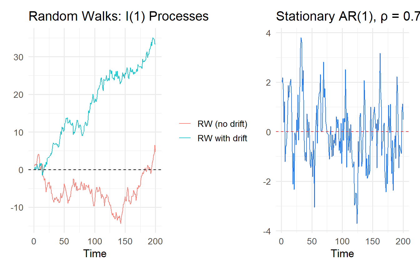
## The Random Walk: Properties Derived
A **random walk** is the canonical I(1) process:
$$y_t = y_{t-1} + e_t, \qquad e_t \sim \text{i.i.d.}(0, \sigma^2), \quad y_0 = 0$$
### Derivation of Properties
**Starting from the recursive structure.** Unrolling the recursion:
$$y_t = y_{t-1} + e_t = y_{t-2} + e_{t-1} + e_t = \cdots = y_0 + \sum_{s=1}^t e_s = \sum_{s=1}^t e_s$$
**Mean:**
$$E[y_t] = E\!\left[\sum_{s=1}^t e_s\right] = \sum_{s=1}^t E[e_s] = 0 \quad \text{for all } t$$
The mean is zero (or $y_0$ if $y_0 \neq 0$). This satisfies condition 1 of weak stationarity (constant mean).
**Variance:**
$$\text{Var}(y_t) = \text{Var}\!\left(\sum_{s=1}^t e_s\right) = \sum_{s=1}^t \text{Var}(e_s) = t\sigma^2$$
The variance **grows linearly with $t$**. This violates condition 2 of weak stationarity. As $t \to \infty$, $\text{Var}(y_t) \to \infty$.
**Autocovariance.** For $h \geq 0$:
$$\text{Cov}(y_t, y_{t+h}) = \text{Cov}\!\left(\sum_{s=1}^t e_s,\; \sum_{r=1}^{t+h} e_r\right) = \sum_{s=1}^t \sum_{r=1}^{t+h} \text{Cov}(e_s, e_r) = t\sigma^2$$
(Only the $s = r \leq t$ terms contribute, since $e_s$ are independent.) The autocovariance depends on $t$ (not just $h$), violating condition 3.
**Autocorrelation:**
$$\text{Corr}(y_t, y_{t+h}) = \frac{t\sigma^2}{\sqrt{t\sigma^2 \cdot (t+h)\sigma^2}} = \sqrt{\frac{t}{t+h}} \to 1 \text{ as } t \to \infty$$
For large $t$, consecutive values are nearly perfectly correlated — the series has **infinite memory** (shocks are permanent).
::: {.callout-important}
## Summary: Random Walk Stationarity Violations
1. Mean: $E[y_t] = 0$ — **satisfies** condition 1 ✓
2. Variance: $\text{Var}(y_t) = t\sigma^2 \to \infty$ — **violates** condition 2 ✗
3. Autocovariance: $\text{Cov}(y_t, y_{t+h}) = t\sigma^2$ (depends on $t$) — **violates** condition 3 ✗
:::
### Random Walk with Drift
A **random walk with drift** adds a constant:
$$y_t = \mu + y_{t-1} + e_t = y_0 + \mu t + \sum_{s=1}^t e_s$$
The mean $E[y_t] = y_0 + \mu t$ now grows (or falls) without bound — a **deterministic trend** on top of the stochastic trend. This is I(1) with a non-zero drift, which is important for the ADF specification.
```{r}
#| label: fig-random-walk
#| fig-cap: "Random walks (no mean reversion) vs. stationary AR(1) (mean-reverting)."
T_obs <- 200

sim_data <- tibble(t = 1:T_obs) |>
  mutate(
    rw_nodrift = cumsum(rnorm(T_obs)),
    rw_drift   = 0.1 * 1:T_obs + cumsum(rnorm(T_obs)),
    ar1        = {
      x <- numeric(T_obs); e <- rnorm(T_obs); x[1] <- e[1]
      for (i in 2:T_obs) x[i] <- 0.7 * x[i-1] + e[i]; x
    }
  )

p1 <- sim_data |>
  pivot_longer(c(rw_nodrift, rw_drift), names_to = "series", values_to = "y") |>
  mutate(series = if_else(series == "rw_nodrift", "RW (no drift)", "RW with drift")) |>
  ggplot(aes(t, y, colour = series)) +
  geom_line(alpha = 0.9) +
  geom_hline(yintercept = 0, linetype = "dashed") +
  labs(title = "Random Walks: I(1) Processes", x = "Time", y = NULL, colour = NULL)

p2 <- ggplot(sim_data, aes(t, ar1)) +
  geom_line(colour = "#2c7be5") +
  geom_hline(yintercept = 0, colour = "#e63946", linetype = "dashed") +
  labs(title = "Stationary AR(1), ρ = 0.7", x = "Time", y = NULL)

library(patchwork)
p1 + p2
```
---
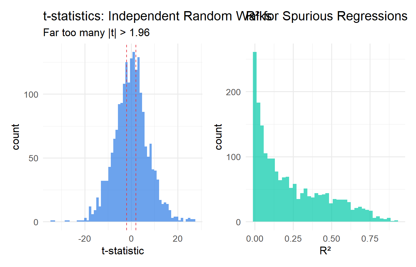
## Spurious Regression
If two independent random walks are regressed on each other, we frequently observe **high $R^2$ and significant $t$-statistics** even though the true relationship is zero. This is **spurious regression**.
**Why does it happen?** Both series accumulate their innovations ($y_t = \sum e_s$, $x_t = \sum v_s$) and so both drift over time. Any finite sample will show some common drift by chance, producing a non-zero sample correlation. The problem is that this sample correlation does not converge to zero as $T \to \infty$ — it converges to a non-degenerate random variable (a ratio of functionals of Brownian motion). Standard $t$-statistics diverge at rate $\sqrt{T}$ rather than converging to a standard normal.
```{r}
#| label: fig-spurious
#| fig-cap: "Spurious regression: t-statistics and R² for pairs of independent random walks."
n_sims  <- 2000
T_obs   <- 100

spurious_results <- map_dfr(1:n_sims, function(i) {
  y <- cumsum(rnorm(T_obs)); x <- cumsum(rnorm(T_obs))
  fit <- lm(y ~ x)
  tibble(t_stat = tidy(fit)$statistic[2], r2 = glance(fit)$r.squared)
})

p_t <- ggplot(spurious_results, aes(t_stat)) +
  geom_histogram(bins = 60, fill = "#2c7be5", alpha = 0.7) +
  geom_vline(xintercept = c(-1.96, 1.96), colour = "#e63946",
             linetype = "dashed") +
  labs(x = "t-statistic", title = "t-statistics: Independent Random Walks",
       subtitle = "Far too many |t| > 1.96")

p_r2 <- ggplot(spurious_results, aes(r2)) +
  geom_histogram(bins = 40, fill = "#00c9a7", alpha = 0.7) +
  labs(x = "R²", title = "R² for Spurious Regressions")

p_t + p_r2
```
```{r}
#| label: spurious-rate
cat("Rejection rate at 5% (nominal):", round(mean(abs(spurious_results$t_stat) > 1.96)*100, 1), "%\n")
cat("Mean R²:", round(mean(spurious_results$r2), 3), "\n")
```
::: {.callout-important}
## Diagnosing Spurious Regression
1. Strongly trended series with very high $R^2$
2. Durbin-Watson statistic close to 0 (residuals themselves are highly autocorrelated — an I(1) residual)
3. "Significant" t-statistics that evaporate when variables are first-differenced
:::
---
## Testing for Unit Roots
### The Dickey-Fuller (DF) Test: Derivation
The DF test is derived directly from the AR(1) model. Consider:
$$y_t = \rho y_{t-1} + e_t$$
**Null hypothesis:** $\rho = 1$ (unit root, I(1)).
**Alternative hypothesis:** $|\rho| < 1$ (stationary, I(0)).
To make the test more convenient, **subtract $y_{t-1}$ from both sides**:
$$y_t - y_{t-1} = (\rho - 1) y_{t-1} + e_t$$
$$\Delta y_t = \theta y_{t-1} + e_t, \qquad \theta = \rho - 1$$
Now $H_0: \theta = 0$ (i.e., $\rho = 1$) and $H_1: \theta < 0$ (i.e., $\rho < 1$). This is a one-sided test in $\theta$.
**Why not just test $\rho = 1$ in the AR(1) directly?** The $t$-statistic for $\hat{\rho} = 1$ does not have a standard normal or $t$-distribution under $H_0$, because when $\rho = 1$, the regressor $y_{t-1}$ is non-stationary — the usual asymptotic theory (which requires stationarity of regressors) breaks down. The DF test uses this reparameterisation so that $H_0: \theta = 0$ can be directly stated, but the distribution of the test statistic under $H_0$ must be simulated (it is the "Dickey-Fuller distribution").
### Three DF Model Variants
The choice of deterministic components in the DF regression matters for the power and size of the test. There are three standard specifications:
**Model 1 — No constant, no trend:**
$$\Delta y_t = \theta y_{t-1} + e_t$$
Use only if the series has zero mean under both $H_0$ and $H_1$. Almost never appropriate in practice.
**Model 2 — Constant (drift), no trend:**
$$\Delta y_t = \alpha + \theta y_{t-1} + e_t$$
Appropriate when $y_t$ may have a non-zero mean but no trend under $H_1$. The most common specification for economic series that are stationary around a constant.
**Model 3 — Constant + trend:**
$$\Delta y_t = \alpha + \beta t + \theta y_{t-1} + e_t$$
Appropriate when $y_t$ may have a deterministic trend under $H_1$ (i.e., $y_t$ is trend-stationary rather than difference-stationary). Use when the series clearly trends upward or downward.
Each variant has **different critical values** — more negative in the more general models.
### Why Are ADF Critical Values Non-Standard?
Under $H_0: \theta = 0$ (i.e., $y_t$ is a random walk), the regressor $y_{t-1}$ is non-stationary — it has variance growing as $t\sigma^2$. The OLS estimator $\hat{\theta}$ is:
$$\hat{\theta} = \frac{\sum_{t=2}^T \Delta y_t \cdot y_{t-1}}{\sum_{t=2}^T y_{t-1}^2}$$
Under the unit root null, $y_{t-1}/\sqrt{T}$ converges to a **Brownian motion** $W(r)$. The numerator and denominator, when appropriately normalised, converge to stochastic integrals of Brownian motion. The limiting distribution of $\hat{\theta} / \text{se}(\hat{\theta})$ (the DF statistic $\tau$) is:
$$\tau \xrightarrow{d} \frac{\int_0^1 W(r)\, dW(r)}{\sqrt{\int_0^1 W(r)^2\, dr}}$$
This distribution is skewed to the left and more negative than the standard $t$. Critical values must be obtained from simulation (Dickey and Fuller 1979, MacKinnon 1996). For the constant-only model with $T \to \infty$, the 5% critical value is approximately $-2.86$ (compared to $-1.65$ for a standard one-sided 5% $t$-test).
### The Augmented Dickey-Fuller (ADF) Test
The basic DF test assumes $e_t$ is i.i.d., but in practice, regression errors are often serially correlated. The **ADF test** augments the DF regression with lagged differences $\Delta y_{t-j}$ to "whiten" the errors:
$$\Delta y_t = \alpha + \beta t + \theta y_{t-1} + \sum_{j=1}^p \gamma_j \Delta y_{t-j} + e_t$$
The lag length $p$ is selected by AIC or BIC. The test statistic is still $\hat{\theta} / \text{se}(\hat{\theta})$, with the same (simulated) critical values.
```{r}
#| label: adf-tests
# ADF on inflation (expect I(0))
cat("--- Inflation (should be I(0)) ---\n")
adf_inf <- adf.test(phillips$inf, alternative = "stationary")
print(adf_inf)
# ADF on interest rate level (may be I(1))
cat("\n--- 3-month T-bill rate: levels (may be I(1)) ---\n")
adf_i3_lev <- adf.test(intdef$i3, alternative = "stationary")
print(adf_i3_lev)
# ADF on first-differenced interest rate (should become I(0))
cat("\n--- 3-month T-bill rate: first difference (should be I(0)) ---\n")
adf_i3_diff <- adf.test(diff(intdef$i3), alternative = "stationary")
print(adf_i3_diff)
```
::: {.callout-tip}
## Practical ADF Protocol
1. Plot the series — look for trends, drifts, breaks
2. Choose model variant (constant only vs. constant + trend)
3. Select lag length by AIC/BIC (or use `adf.test()` with automatic lag selection)
4. Compare the ADF statistic to the appropriate critical value (not standard $t$-critical values!)
5. If fail to reject in levels, first-difference and retest to confirm I(0) after differencing
:::
---
## The KPSS Test
The **KPSS test** reverses the null and alternative relative to the ADF:
- $H_0$: series is stationary (I(0))
- $H_1$: series has a unit root (I(1))
The KPSS test statistic is based on cumulative sums of residuals from a regression of $y_t$ on a constant (or constant + trend). It is constructed as:
$$KPSS = \frac{1}{T^2 \hat{\sigma}^2} \sum_{t=1}^T S_t^2, \qquad S_t = \sum_{s=1}^t \hat{e}_s$$
where $\hat{e}_t$ are residuals from the null model and $\hat{\sigma}^2$ is the long-run variance estimate. Under $H_0$, $KPSS \to \int_0^1 V(r)^2\, dr$ (a function of a standard Brownian bridge), giving the non-standard critical values.
**Using ADF and KPSS together:**
| ADF | KPSS | Conclusion |
|---|---|---|
| Reject $H_0$ | Fail to reject $H_0$ | Strong evidence of **stationarity** |
| Fail to reject $H_0$ | Reject $H_0$ | Strong evidence of **unit root** |
| Fail to reject $H_0$ | Fail to reject $H_0$ | Cannot distinguish — low power |
| Reject $H_0$ | Reject $H_0$ | Contradiction — check for structural breaks |
```{r}
#| label: kpss-test
cat("KPSS: inf (H0: stationary)\n"); print(kpss.test(phillips$inf, null = "Level"))
cat("KPSS: i3 (H0: stationary)\n"); print(kpss.test(intdef$i3, null = "Level"))
cat("KPSS: diff(i3)\n"); print(kpss.test(diff(intdef$i3), null = "Level"))
```
---
## What to Do with Non-Stationary Series
### Option 1: First-Difference
If $y_t$ and $x_t$ are both I(1) and **not cointegrated**, regress $\Delta y_t$ on $\Delta x_t$. This restores stationarity and valid inference but sacrifices information about the **long-run** level relationship.
```{r}
#| label: first-difference
fit_levels <- lm(i3 ~ inf + def, data = intdef)

intdef_diff <- intdef |>
  mutate(d_i3 = c(NA, diff(i3)), d_inf = c(NA, diff(inf)), d_def = c(NA, diff(def))) |>
  drop_na()

fit_diff <- lm(d_i3 ~ d_inf + d_def, data = intdef_diff)

modelsummary(
  list("Levels (potentially spurious)" = fit_levels, "First differences" = fit_diff),
  stars = TRUE, gof_map = c("nobs", "r.squared"),
  title = "Levels vs. First Differences: Interest Rate Model"
)
```
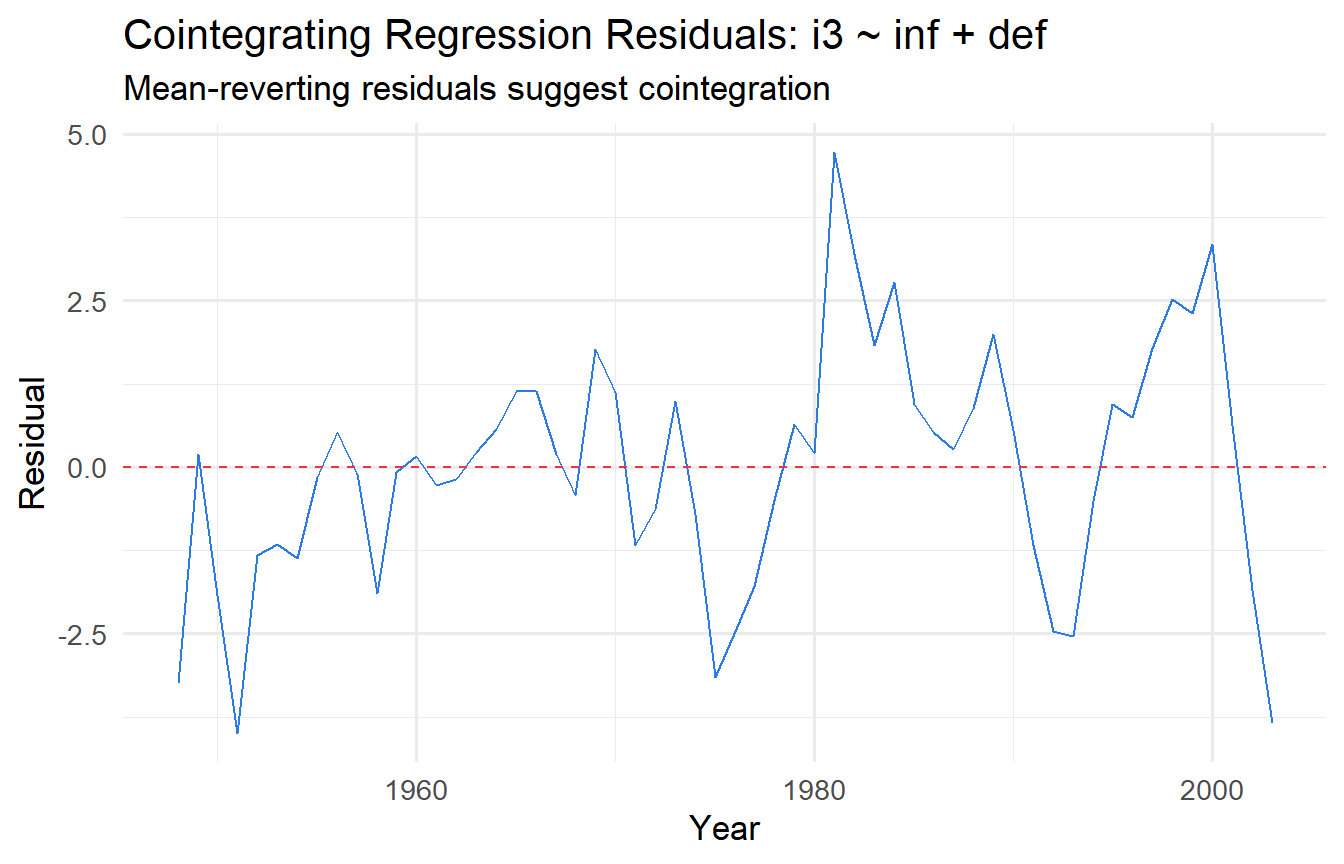
### Option 2: Cointegration and the Engle-Granger Two-Step Procedure
Two I(1) series are **cointegrated** if there exists a linear combination $y_t - \beta x_t$ that is I(0). In this case, the series share a **common stochastic trend** — they cannot drift apart indefinitely. Regressing $y_t$ on $x_t$ in levels recovers the **long-run equilibrium relationship** and is called the **cointegrating regression**.
**Engle-Granger two-step procedure:**
**Step 1.** Estimate the cointegrating regression by OLS:
$$y_t = \beta_0 + \beta_1 x_t + v_t$$
Obtain the residuals $\hat{v}_t = y_t - \hat{\beta}_0 - \hat{\beta}_1 x_t$.
**Step 2.** Test whether $\hat{v}_t$ is I(0) using an ADF test.
If the ADF rejects for the residuals, conclude cointegration. **Important:** the critical values for this second-stage ADF test are **more negative** than standard ADF critical values, because we are testing on estimated (not true) residuals. The MacKinnon (1991) critical values for the Engle-Granger test with one regressor are approximately:
| Significance level | 1% | 5% | 10% |
|---|---|---|---|
| Critical value (T→∞) | −3.90 | −3.34 | −3.04 |
These are more negative than the corresponding single-series ADF critical values ($-3.43$, $-2.86$, $-2.57$), because estimating $\beta$ in Step 1 introduces additional uncertainty.
```{r}
#| label: cointegration-test
# Step 1: Cointegrating regression
fit_coint <- lm(i3 ~ inf + def, data = intdef)
resid_coint <- residuals(fit_coint)

# Step 2: ADF on residuals (Engle-Granger test)
cat("Engle-Granger test (ADF on residuals):\n")
eg_test <- adf.test(resid_coint, alternative = "stationary")
print(eg_test)
# Visualise residuals
tibble(year = intdef$year, resid = resid_coint) |>
  ggplot(aes(year, resid)) +
  geom_line(colour = "#2c7be5") +
  geom_hline(yintercept = 0, linetype = "dashed", colour = "#e63946") +
  labs(x = "Year", y = "Residual",
       title = "Cointegrating Regression Residuals: i3 ~ inf + def",
       subtitle = "Mean-reverting residuals suggest cointegration")
```
::: {.callout-important}
## Engle-Granger Critical Values
Use the MacKinnon critical values ($-3.34$ at 5% for one cointegrating variable), not the standard ADF critical values ($-2.86$). Failing to use the correct critical values leads to over-rejection of the null of no cointegration — incorrectly concluding that a spurious long-run relationship is genuine.
:::
### Error Correction Models (ECM)
When cointegration is present, the **Granger representation theorem** guarantees an ECM representation. For variables cointegrated as $y_t \approx \beta x_t$:
$$\Delta y_t = \alpha_0 + \alpha_1 \Delta x_t + \lambda (y_{t-1} - \hat{\beta} x_{t-1}) + e_t$$
The term $y_{t-1} - \hat{\beta} x_{t-1}$ is the **error correction term** — the lagged deviation from the long-run equilibrium. $\lambda < 0$ ensures deviations are corrected: if $y_{t-1}$ is above its long-run level, $\Delta y_t$ will be pulled downward.
**Derivation from ADL.** Start with an ADL(1,1):
$$y_t = \delta_0 + \rho y_{t-1} + \gamma_0 x_t + \gamma_1 x_{t-1} + e_t$$
Subtract $y_{t-1}$ from both sides:
$$\Delta y_t = \delta_0 + (\rho - 1)y_{t-1} + \gamma_0 \Delta x_t + (\gamma_0 + \gamma_1)x_{t-1} + e_t$$
$$= \delta_0 + \gamma_0 \Delta x_t + (\rho-1)\!\left[y_{t-1} - \frac{\gamma_0 + \gamma_1}{\rho - 1} x_{t-1}\right] + e_t \quad (\text{rearranging})$$
Setting $\lambda = \rho - 1 < 0$ and $\beta_{LR} = -(\gamma_0 + \gamma_1)/(\rho - 1) = (\gamma_0 + \gamma_1)/(1-\rho)$ gives the ECM with the long-run coefficient $\beta_{LR}$.
```{r}
#| label: ecm
# Two-step Engle-Granger ECM
# Step 1: Cointegrating regression
fit_step1 <- lm(i3 ~ inf, data = intdef)
intdef_ecm <- intdef |>
  mutate(
    ecm_lag = lag(residuals(fit_step1)),
    d_i3    = c(NA, diff(i3)),
    d_inf   = c(NA, diff(inf))
  ) |>
  drop_na()

# Step 2: ECM
fit_ecm <- lm(d_i3 ~ d_inf + ecm_lag, data = intdef_ecm)
tidy(fit_ecm, conf.int = TRUE)
```
The `ecm_lag` coefficient $\hat{\lambda}$ should be negative and significant — confirming error correction. Its magnitude tells us the fraction of the deviation from equilibrium corrected each period.
---
## Tutorials
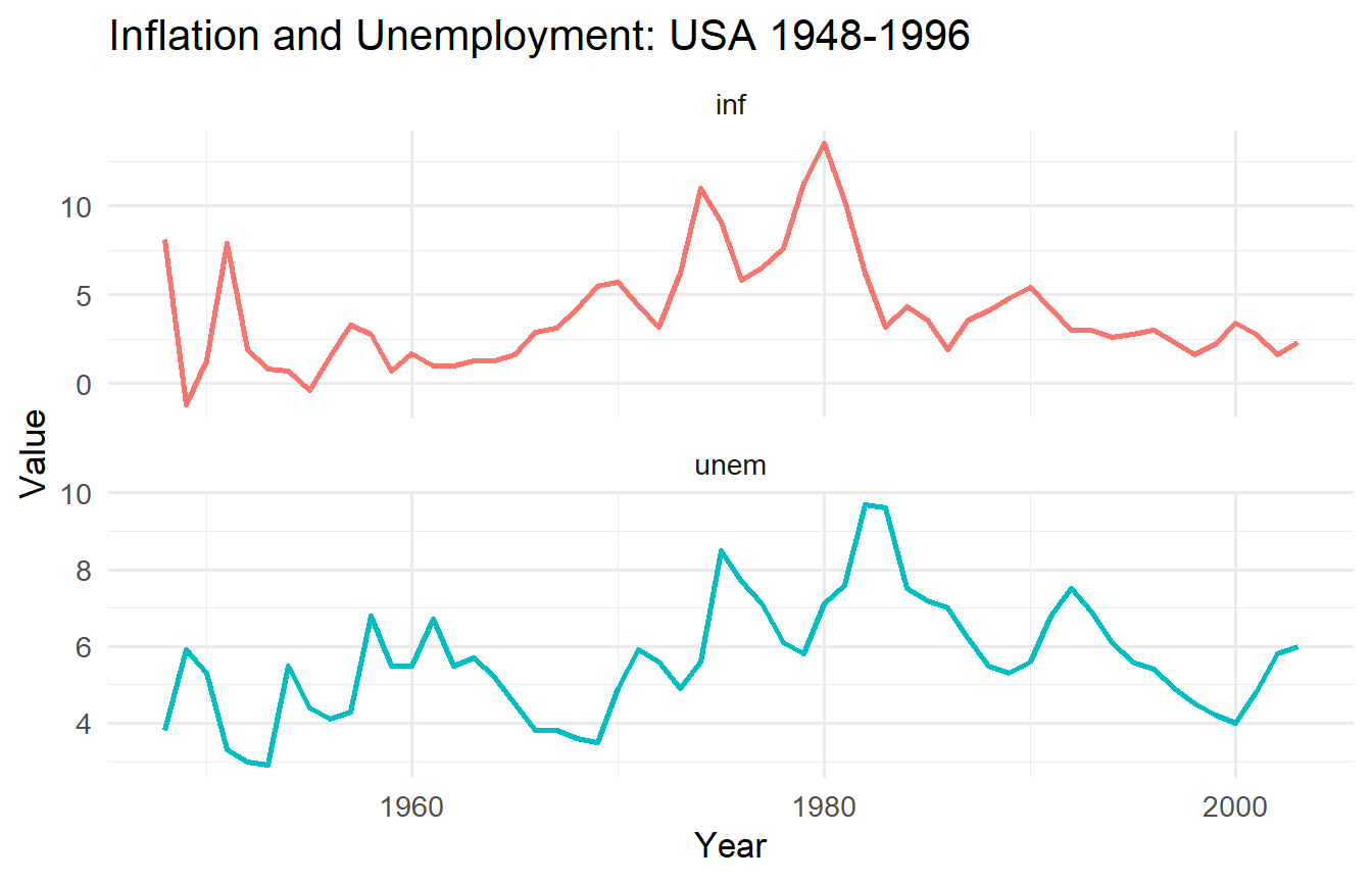
**Tutorial 12.1**
Using `wooldridge::phillips`, test whether `inf` and `unem` are I(0) or I(1).
a. Plot both series. Do they appear stationary?
b. Apply the ADF test (with constant, no trend) to each in levels and first differences. Compare ADF statistics to the 5% critical value of $-2.86$.
c. Apply the KPSS test. Are ADF and KPSS conclusions consistent?
::: {.callout-tip collapse="true"}
## Solution
```{r}
#| label: ex12-1
phillips_long <- phillips |>
  pivot_longer(c(inf, unem), names_to = "variable", values_to = "value")

ggplot(phillips_long, aes(year, value, colour = variable)) +
  geom_line(linewidth = 1) +
  facet_wrap(~ variable, scales = "free_y", ncol = 1) +
  labs(x = "Year", y = "Value", title = "Inflation and Unemployment: USA 1948-1996") +
  theme(legend.position = "none")
for (var in c("inf", "unem")) {
  cat("\n---", var, "levels ---\n")
  print(adf.test(phillips[[var]]))
  cat("---", var, "first diff ---\n")
  print(adf.test(diff(phillips[[var]])))
  cat("--- KPSS:", var, "---\n")
  print(kpss.test(phillips[[var]], null = "Level"))
}
```
Inflation is typically found borderline stationary — the ADF may or may not reject at 5% depending on lag length. Unemployment shows stronger evidence of a unit root in this sample. The sensitivity to sample period and lag selection is a real challenge with unit root tests in short macroeconomic time series.
:::
**Tutorial 12.2**
Demonstrate the spurious regression problem using simulation.
a. Generate 1,000 pairs of independent random walks ($T = 100$). Record the t-statistic and $R^2$ from each regression.
b. Repeat with two independent I(0) AR(1) processes ($\rho = 0.5$).
c. Compare rejection rates at the 5% nominal level and mean $R^2$ values.
::: {.callout-tip collapse="true"}
## Solution
```{r}
#| label: ex12-2
T_obs  <- 100
n_sims <- 1000

sim_t <- function(rw = TRUE) {
  map_dfr(1:n_sims, function(i) {
    if (rw) {
      y <- cumsum(rnorm(T_obs)); x <- cumsum(rnorm(T_obs))
    } else {
      y <- as.numeric(arima.sim(list(ar = 0.5), n = T_obs))
      x <- as.numeric(arima.sim(list(ar = 0.5), n = T_obs))
    }
    fit <- lm(y ~ x)
    tibble(t_stat = tidy(fit)$statistic[2], r2 = glance(fit)$r.squared)
  })
}

res_rw  <- sim_t(rw = TRUE)
res_ar1 <- sim_t(rw = FALSE)

cat("Random Walk  — Rejection rate:", round(mean(abs(res_rw$t_stat) > 1.96), 3),
    "  Mean R²:", round(mean(res_rw$r2), 3), "\n")
cat("AR(1), ρ=0.5 — Rejection rate:", round(mean(abs(res_ar1$t_stat) > 1.96), 3),
    "  Mean R²:", round(mean(res_ar1$r2), 3), "\n")
```
The random walk regression rejects far above 5% with inflated $R^2$. The stationary AR(1) regression rejects close to 5% with low average $R^2$, confirming valid inference for stationary processes.
:::
**Tutorial 12.3**
Using `wooldridge::intdef`, apply the Engle-Granger two-step procedure to test for cointegration between `i3` and `inf`.
a. Confirm `i3` and `inf` are I(1) using ADF tests.
b. Estimate the cointegrating regression `i3 ~ inf`.
c. Apply the ADF test to the residuals. Compare the ADF statistic to the Engle-Granger 5% critical value of $-3.34$ (not $-2.86$).
d. If cointegrated, estimate the ECM. Interpret $\hat{\lambda}$ (the speed of adjustment).
::: {.callout-tip collapse="true"}
## Solution
```{r}
#| label: ex12-3
# a) Unit root tests
cat("ADF: i3\n");  print(adf.test(intdef$i3))
cat("ADF: inf\n"); print(adf.test(intdef$inf))
# b) Cointegrating regression
fit_coint2 <- lm(i3 ~ inf, data = intdef)
cat("\nCointegrating regression:\n"); tidy(fit_coint2)
# c) ADF on residuals with EG critical values
resid2 <- residuals(fit_coint2)
cat("\nEngle-Granger test (ADF on residuals):\n")
eg2 <- adf.test(resid2, alternative = "stationary")
print(eg2)
cat("EG 5% critical value: -3.34\n")
cat("Conclusion:", if (eg2$statistic < -3.34) "Reject H0 (cointegrated)" else "Fail to reject (not cointegrated)", "\n")
# d) ECM
intdef_ecm2 <- intdef |>
  mutate(ecm_lag = lag(resid2), d_i3 = c(NA, diff(i3)), d_inf = c(NA, diff(inf))) |>
  drop_na()

fit_ecm2 <- lm(d_i3 ~ d_inf + ecm_lag, data = intdef_ecm2)
tidy(fit_ecm2)
```
The Fisher effect implies a long-run one-for-one relationship between nominal interest rates and inflation. If cointegrated, $\hat{\lambda}$ measures the fraction of any deviation from the long-run equilibrium that is corrected each period (year). A value of $\hat{\lambda} \approx -0.3$ would mean 30% of the deviation is corrected annually.
:::