---
title: "Chapter 3: Simple Linear Regression"
subtitle: "OLS estimation, matrix form, geometry, and goodness of fit"
---
```{r}
#| label: setup
#| include: false
library(tidyverse)
library(broom)
library(modelsummary)
library(patchwork)
library(wooldridge)
theme_set(theme_minimal(base_size = 13))
options(digits = 4, scipen = 999)
```
::: {.callout-note}
## Learning Objectives
By the end of this chapter you will be able to:
- State the simple linear regression model and interpret its components
- Derive the OLS estimator algebraically from first-order conditions
- Write the regression model and the OLS estimator in matrix form
- Explain OLS geometrically as an orthogonal projection onto the column space of $\mathbf{X}$
- Derive the normal equations $\mathbf{X'X}\hat{\boldsymbol{\beta}} = \mathbf{X'y}$ from the orthogonality principle
- Verify the algebraic properties of OLS residuals
- Derive the SST = SSE + SSR decomposition as a consequence of orthogonality
- Compute and interpret $R^2$ and the standard error of the regression
- Fit and interpret a regression model in R
:::
---
## The Population Regression Function
We want to understand how a variable $y$ (the **dependent variable**) relates to $x$ (the **independent variable** or **regressor**). The population model is:
$$
y_i = \beta_0 + \beta_1 x_i + u_i, \quad i = 1, 2, \ldots, n
$$
- $\beta_0$: the **intercept** — expected value of $y$ when $x = 0$
- $\beta_1$: the **slope** — the change in $y$ per unit increase in $x$, ceteris paribus
- $u_i$: the **error term** — all factors that determine $y$ other than $x$
The interpretation $\Delta y / \Delta x = \beta_1$ is valid only when $\Delta u / \Delta x = 0$: that is, when $x$ changes do not move the unobservables. This is the **ceteris paribus** requirement.
### The Population Regression Function
The **zero conditional mean assumption** $E[u \mid x] = 0$ implies:
$$
E[y \mid x] = \beta_0 + \beta_1 x
$$
This is the **population regression function (PRF)**. It describes the true conditional mean in the population. We never observe it; we estimate it from data. Estimating the PRF requires a random sample $\{(x_i, y_i) : i = 1, \ldots, n\}$.
### SLR Assumptions
| | Assumption | Statement |
|--|-----------|-----------|
| **SLR.1** | Linearity | $y = \beta_0 + \beta_1 x + u$ |
| **SLR.2** | Random sampling | $(x_i, y_i)$ are i.i.d. draws from the population |
| **SLR.3** | Sample variation in $x$ | $\sum(x_i - \bar{x})^2 > 0$ |
| **SLR.4** | Zero conditional mean | $E[u \mid x] = 0$ |
SLR.4 is the load-bearing assumption. Its violation produces **endogeneity** and makes $\hat{\beta}_1$ biased.
### What Is a Model?
Studying two random variables means modelling their joint distribution — which is data-intensive. The strategy here is more targeted: model the **conditional distribution** of $y$ given $x$, and in particular its conditional mean $E[y \mid x]$.
An **incomplete model** specifies only $E[y \mid x] = \beta_0 + \beta_1 x$. A **complete model** (the **Classical Linear Model**) further specifies:
$$
\text{Var}(u \mid x) = \sigma^2 \quad \text{(homoskedasticity)}
$$
$$
u \mid x \sim \mathcal{N}(0, \sigma^2) \quad \text{(normality)}
$$
this chapter we work with the incomplete model. The CLM assumptions are taken up in Chapters 4 and 5.
---
## OLS Estimation: Scalar Derivation
Given data $(x_1, y_1), \ldots, (x_n, y_n)$, we need to choose $\hat{\beta}_0$ and $\hat{\beta}_1$. OLS chooses the values that minimise the **sum of squared residuals**:
$$
\min_{b_0,\, b_1} \; S(b_0, b_1) = \sum_{i=1}^{n} (y_i - b_0 - b_1 x_i)^2
$$
**First-order conditions:**
$$
\frac{\partial S}{\partial b_0}\bigg|_{\hat{\beta}} = -2\sum_{i=1}^{n}(y_i - \hat{\beta}_0 - \hat{\beta}_1 x_i) = 0
$$
$$
\frac{\partial S}{\partial b_1}\bigg|_{\hat{\beta}} = -2\sum_{i=1}^{n} x_i(y_i - \hat{\beta}_0 - \hat{\beta}_1 x_i) = 0
$$
These two equations — the **normal equations** in scalar form — are:
$$
\sum_{i=1}^{n} \hat{u}_i = 0 \tag{1}
$$
$$
\sum_{i=1}^{n} x_i \hat{u}_i = 0 \tag{2}
$$
**Solving the system.** Dividing (1) by $n$ gives $\hat{\beta}_0 = \bar{y} - \hat{\beta}_1 \bar{x}$. Substituting into (2) and simplifying (see Wooldridge p. 28):
$$
\boxed{\hat{\beta}_1 = \frac{\sum_{i=1}^n (x_i - \bar{x})(y_i - \bar{y})}{\sum_{i=1}^n (x_i - \bar{x})^2} = \frac{\widehat{\text{Cov}}(x, y)}{\widehat{\text{Var}}(x)}}
$$
$$
\boxed{\hat{\beta}_0 = \bar{y} - \hat{\beta}_1 \bar{x}}
$$
Notice that $\hat{\beta}_1 = \hat{\sigma}_{xy} / \hat{\sigma}_x^2$: the OLS slope is the sample covariance of $x$ and $y$ divided by the sample variance of $x$. In finance, this same formula gives the market **beta** of a stock.
The **estimated regression line** is $\hat{y} = \hat{\beta}_0 + \hat{\beta}_1 x$. Since $\hat{\beta}_0 = \bar{y} - \hat{\beta}_1 \bar{x}$, the line always passes through the sample mean $(\bar{x}, \bar{y})$.
### Estimators We Have Seen
Every population moment has a sample analogue. The table below collects them:
| Population parameter | Estimator |
|---|---|
| $\mu_y = E[y]$ | $\bar{y} = \frac{1}{n}\sum y_i$ |
| $\sigma_y^2 = E[(y - \mu_y)^2]$ | $\hat{s}_y^2 = \frac{1}{n-1}\sum(y_i - \bar{y})^2$ |
| $\sigma_{xy} = E[(x-\mu_x)(y-\mu_y)]$ | $\hat{s}_{xy} = \frac{1}{n-1}\sum(x_i - \bar{x})(y_i - \bar{y})$ |
| $\rho_{xy} = \sigma_{xy}/(\sigma_x \sigma_y)$ | $\hat{r}_{xy} = \hat{s}_{xy}/(\hat{s}_x \hat{s}_y)$ |
| $\beta_1$ in $E[y\mid x] = \beta_0 + \beta_1 x$ | $\hat{\beta}_1 = \hat{s}_{xy}/\hat{s}_x^2$ |
| $\beta_0$ | $\hat{\beta}_0 = \bar{y} - \hat{\beta}_1\bar{x}$ |
In every case the estimator is a function of sample data only. Because the data are random, $\hat{\beta}_0$ and $\hat{\beta}_1$ are **random variables**: different samples from the same population will yield different estimates.
---
## Matrix Form of the Regression Model
For $n$ observations the model $y_i = \beta_0 + \beta_1 x_i + u_i$ for $i = 1, \ldots, n$ can be stacked:
$$
\underbrace{\begin{bmatrix} y_1 \\ y_2 \\ \vdots \\ y_n \end{bmatrix}}_{\mathbf{y} \; (n \times 1)}
=
\underbrace{\begin{bmatrix} 1 & x_1 \\ 1 & x_2 \\ \vdots & \vdots \\ 1 & x_n \end{bmatrix}}_{\mathbf{X} \; (n \times 2)}
\underbrace{\begin{bmatrix} \beta_0 \\ \beta_1 \end{bmatrix}}_{\boldsymbol{\beta} \; (2 \times 1)}
+
\underbrace{\begin{bmatrix} u_1 \\ u_2 \\ \vdots \\ u_n \end{bmatrix}}_{\mathbf{u} \; (n \times 1)}
$$
Compactly: $\mathbf{y} = \mathbf{X}\boldsymbol{\beta} + \mathbf{u}$.
The first column of $\mathbf{X}$ is a column of ones, which "carries" the intercept $\beta_0$. The matrix $\mathbf{X}$ and vector $\mathbf{y}$ are **observable**; $\boldsymbol{\beta}$ and $\mathbf{u}$ are **unobservable**.
### Extension to Multiple Regression
With $k$ regressors plus an intercept the model is identical in form:
$$
\mathbf{y} = \mathbf{X}\boldsymbol{\beta} + \mathbf{u}, \quad \mathbf{X} \in \mathbb{R}^{n \times (k+1)}, \quad \boldsymbol{\beta} \in \mathbb{R}^{k+1}
$$
The power of abstraction: four apparently distinct problems — returns to education, stock betas, house price prediction, electricity load forecasting — are all instances of the single problem "estimate $\boldsymbol{\beta}$ in $\mathbf{y} = \mathbf{X}\boldsymbol{\beta} + \mathbf{u}$ from a sample of observations."
---
## Geometry of OLS
This section gives the geometric interpretation of least squares. It is not in Wooldridge but is essential for understanding what OLS computes, why $\mathbf{X'\hat{u}} = \mathbf{0}$, and where the $SST = SSE + SSR$ decomposition comes from.
### Vectors and Inner Products
Think of $\mathbf{y} = (y_1, \ldots, y_n)' \in \mathbb{R}^n$ as a point (or arrow from the origin) in $n$-dimensional space.
**Length** of a vector $\mathbf{v} \in \mathbb{R}^n$:
$$
\|\mathbf{v}\| = \sqrt{\mathbf{v}'\mathbf{v}} = \sqrt{\sum_{i=1}^n v_i^2}
$$
**Orthogonality.** Two vectors $\mathbf{u}, \mathbf{v} \in \mathbb{R}^n$ are **orthogonal** (perpendicular) if and only if:
$$
\mathbf{u}'\mathbf{v} = \sum_{i=1}^n u_i v_i = 0
$$
### The Column Space of $\mathbf{X}$
For any $(k+1)$-vector $\mathbf{b}$, the product $\mathbf{Xb}$ is an $n$-vector that is a **linear combination of the columns of $\mathbf{X}$**. The set of all such vectors:
$$
\mathcal{C}(\mathbf{X}) = \{\mathbf{Xb} : \mathbf{b} \in \mathbb{R}^{k+1}\}
$$
is the **column space** (or **range**) of $\mathbf{X}$. It is a subspace of $\mathbb{R}^n$.
- If $\mathbf{X}$ has $k+1$ **linearly independent** columns, then $\mathcal{C}(\mathbf{X})$ is a $(k+1)$-dimensional flat (hyperplane through the origin) inside $\mathbb{R}^n$.
- With $k+1 < n$ (more observations than parameters — the usual case), this flat is a proper subspace: **$\mathbf{y}$ will generically not lie in $\mathcal{C}(\mathbf{X})$.**
### A Concrete Illustration
**Two observations, two parameters.** Suppose $n = 2$ and $\mathbf{X}$ has two linearly independent columns. Then $\mathcal{C}(\mathbf{X}) = \mathbb{R}^2$: every 2-vector $\mathbf{y}$ lies in $\mathcal{C}(\mathbf{X})$, so we can fit the data perfectly with zero residuals.
**Three observations, two parameters.** Now $n = 3$, $k+1 = 2$. $\mathcal{C}(\mathbf{X})$ is a 2-dimensional plane through the origin in $\mathbb{R}^3$. A generic $\mathbf{y} \in \mathbb{R}^3$ does **not** lie in this plane, so perfect fit is impossible.
```{r}
#| label: house-example
# Three houses: bedrooms = 4, 1, 1; prices = 10, 4, 6 (hundreds of thousands)
y <- c(10, 4, 6)
X <- cbind(1, c(4, 1, 1))   # [intercept | bedrooms]

# OLS: beta_hat = (X'X)^{-1} X'y
beta_hat <- solve(t(X) %*% X) %*% (t(X) %*% y)
y_hat    <- X %*% beta_hat
u_hat    <- y - y_hat

cat("beta_hat:", round(beta_hat, 4), "\n")
cat("y_hat: ", round(y_hat, 4), "\n")
cat("u_hat: ", round(u_hat, 4), "\n")
```
The residuals are non-zero: the data vector $\mathbf{y}$ does not lie in $\mathcal{C}(\mathbf{X})$.
### OLS as Orthogonal Projection
The OLS objective is:
$$
\min_{\mathbf{b}} \|\mathbf{y} - \mathbf{Xb}\|^2 = \min_{\mathbf{b}} \sum_{i=1}^n (y_i - \mathbf{x}_i'\mathbf{b})^2
$$
This is the problem of finding the point in $\mathcal{C}(\mathbf{X})$ **closest to $\mathbf{y}$** in Euclidean distance. The solution is the **orthogonal projection** of $\mathbf{y}$ onto $\mathcal{C}(\mathbf{X})$.
The projection $\hat{\mathbf{y}} = \mathbf{X}\hat{\boldsymbol{\beta}}$ is the unique point in $\mathcal{C}(\mathbf{X})$ such that the residual $\hat{\mathbf{u}} = \mathbf{y} - \hat{\mathbf{y}}$ is **perpendicular to the entire column space**:
$$
\hat{\mathbf{u}} \perp \mathcal{C}(\mathbf{X})
$$
::: {.callout-note}
## The Orthogonality Principle
$$\mathbf{X'}\hat{\mathbf{u}} = \mathbf{0}$$
The OLS residual vector is orthogonal to every column of $\mathbf{X}$. This single equation contains the entire geometry of OLS and is more important than any formula.
:::
The orthogonality condition says: the residual is uncorrelated with every regressor (including the constant). Writing it out column by column for $\mathbf{X} = [\mathbf{1}, \mathbf{x}_1, \ldots, \mathbf{x}_k]$:
$$
\mathbf{1}'\hat{\mathbf{u}} = \sum_{i=1}^n \hat{u}_i = 0
\qquad
\mathbf{x}_j'\hat{\mathbf{u}} = \sum_{i=1}^n x_{ij}\hat{u}_i = 0, \quad j = 1, \ldots, k
$$
These are exactly the scalar normal equations (1) and (2) we derived from the first-order conditions.
```{r}
#| label: orthogonality-check
# Verify X'u_hat = 0 for the house example
round(t(X) %*% u_hat, 10)   # should be (0, 0)
```
### Deriving the OLS Formula
Substituting $\hat{\mathbf{u}} = \mathbf{y} - \mathbf{X}\hat{\boldsymbol{\beta}}$ into $\mathbf{X'}\hat{\mathbf{u}} = \mathbf{0}$:
$$
\mathbf{X}'(\mathbf{y} - \mathbf{X}\hat{\boldsymbol{\beta}}) = \mathbf{0}
$$
$$
\mathbf{X'y} = \mathbf{X'X}\hat{\boldsymbol{\beta}} \tag{Normal Equations}
$$
$$
\boxed{\hat{\boldsymbol{\beta}} = (\mathbf{X'X})^{-1}\mathbf{X'y}}
$$
provided $\mathbf{X'X}$ is invertible — which requires the columns of $\mathbf{X}$ to be **linearly independent** (no perfect multicollinearity).
### The Projection and Annihilator Matrices
Substituting back, the fitted values are:
$$
\hat{\mathbf{y}} = \mathbf{X}\hat{\boldsymbol{\beta}} = \mathbf{X}(\mathbf{X'X})^{-1}\mathbf{X'y} \equiv \mathbf{P}_X \mathbf{y}
$$
where $\mathbf{P}_X = \mathbf{X}(\mathbf{X'X})^{-1}\mathbf{X'}$ is the **hat matrix** (it puts the "hat" on $\mathbf{y}$). The residual vector is:
$$
\hat{\mathbf{u}} = \mathbf{y} - \hat{\mathbf{y}} = (\mathbf{I} - \mathbf{P}_X)\mathbf{y} \equiv \mathbf{M}_X \mathbf{y}
$$
where $\mathbf{M}_X = \mathbf{I} - \mathbf{P}_X$ is the **annihilator matrix**. Both $\mathbf{P}_X$ and $\mathbf{M}_X$ are symmetric and idempotent ($\mathbf{P}_X^2 = \mathbf{P}_X$, $\mathbf{M}_X^2 = \mathbf{M}_X$), and they are orthogonal to each other: $\mathbf{P}_X \mathbf{M}_X = \mathbf{0}$.
```{r}
#| label: projection-matrices
n <- nrow(X)
P <- X %*% solve(t(X) %*% X) %*% t(X)   # hat matrix
M <- diag(n) - P                          # annihilator

# Idempotency: P^2 = P
cat("Max deviation P^2 - P:", max(abs(P %*% P - P)), "\n")
# Orthogonality: P M = 0
cat("Max deviation PM:     ", max(abs(P %*% M)),     "\n")
# y_hat and u_hat via projection
round(P %*% y, 4)   # same as y_hat above
round(M %*% y, 4) # same as u_hat above
```
---
## Algebraic Properties of OLS
The orthogonality conditions $\mathbf{X'}\hat{\mathbf{u}} = \mathbf{0}$ have direct algebraic consequences. Writing out the two columns of $\mathbf{X} = [\mathbf{1}, \mathbf{x}]$:
**Property 1.** $\displaystyle\sum_{i=1}^n \hat{u}_i = 0$
The residuals sum to zero. OLS over-predicts as often as it under-predicts. (Follows from the column of ones being in $\mathbf{X}$.)
**Property 2.** $\displaystyle\sum_{i=1}^n x_i \hat{u}_i = 0$
The residuals are uncorrelated with the regressor in the sample.
**Property 3.** $\bar{y} = \hat{\bar{y}} = \hat{\beta}_0 + \hat{\beta}_1 \bar{x}$
The sample mean of fitted values equals the sample mean of $y$. The estimated regression line passes through $(\bar{x}, \bar{y})$.
```{r}
#| label: ols-properties
data("wage1", package = "wooldridge")
fit <- lm(wage ~ educ, data = wage1)
u   <- residuals(fit)
x   <- wage1$educ

cat("Sum of residuals:       ", round(sum(u), 10),       "\n")
cat("Cov(x, u_hat): ", round(sum(x * u), 10), "\n")
cat("Mean(y_hat) == mean(y): ",
    isTRUE(all.equal(mean(fitted(fit)), mean(wage1$wage))), "\n")
```
---
## Goodness of Fit: A Geometric Derivation
Because $\hat{\mathbf{u}} \perp \hat{\mathbf{y}}$ — and because the column of ones in $\mathbf{X}$ forces $\hat{\mathbf{u}} \perp \mathbf{1}$, which means $\bar{\hat{u}} = 0$ and hence $\bar{\hat{y}} = \bar{y}$ — we can work with demeaned vectors.
Define $\tilde{\mathbf{y}} = \mathbf{y} - \bar{y}\mathbf{1}$ and $\tilde{\hat{\mathbf{y}}} = \hat{\mathbf{y}} - \bar{y}\mathbf{1}$. Since $\hat{\mathbf{u}} = \mathbf{y} - \hat{\mathbf{y}}$, we have:
$$
\tilde{\mathbf{y}} = \tilde{\hat{\mathbf{y}}} + \hat{\mathbf{u}}
$$
Squaring both sides (taking inner products) and using $\tilde{\hat{\mathbf{y}}}'\hat{\mathbf{u}} = 0$ (orthogonality — verify: $\hat{\mathbf{y}}'\hat{\mathbf{u}} = \boldsymbol{\beta}'\mathbf{X}'\hat{\mathbf{u}} = 0$):
$$
\|\tilde{\mathbf{y}}\|^2 = \|\tilde{\hat{\mathbf{y}}}\|^2 + \|\hat{\mathbf{u}}\|^2
$$
$$
\underbrace{\sum_{i=1}^n (y_i - \bar{y})^2}_{SST}
= \underbrace{\sum_{i=1}^n (\hat{y}_i - \bar{y})^2}_{SSE}
+ \underbrace{\sum_{i=1}^n \hat{u}_i^2}_{SSR}
$$
This is the **Pythagorean theorem applied to the OLS decomposition** — it holds as an algebraic identity, not as an approximation, and follows directly from orthogonality.
::: {.callout-note}
## Coefficient of Determination
$$R^2 = \frac{SSE}{SST} = 1 - \frac{SSR}{SST}$$
$R^2$ is the squared cosine of the angle between $\tilde{\mathbf{y}}$ and $\tilde{\hat{\mathbf{y}}}$ in $\mathbb{R}^n$. It lies in $[0, 1]$.
:::
::: {.callout-important}
## $R^2$ Does Not Measure Causal Validity
A high $R^2$ does not imply a causal interpretation. The election spending example in Wooldridge has $R^2 = 0.856$ but is still a correlation. The wage–education regression has $R^2 = 0.165$ but its coefficient may be closer to a causal effect (especially after controlling for confounders).
:::
### The Standard Error of the Regression
We need to estimate $\sigma^2 = \text{Var}(u)$. The natural candidate is $SSR/n$, but this is biased because we "used up" $k+1$ degrees of freedom estimating $\boldsymbol{\beta}$. The unbiased estimator is:
$$
\hat{\sigma}^2 = \frac{SSR}{n - (k+1)} = \frac{\sum \hat{u}_i^2}{n - k - 1}
$$
For simple regression ($k = 1$): $\hat{\sigma}^2 = SSR / (n - 2)$.
The **standard error of the regression** (SER) is $\hat{\sigma} = \sqrt{\hat{\sigma}^2}$, reported as `sigma` in `glance()`. It measures residual spread in the units of $y$.
---
## Running Example: Returns to Education
```{r}
#| label: wage1-glimpse
data("wage1", package = "wooldridge")
wage1 |>
  select(wage, educ, exper, female, nonwhite) |>
  datasummary_skim()
```
```{r}
#| label: fig-wage-educ
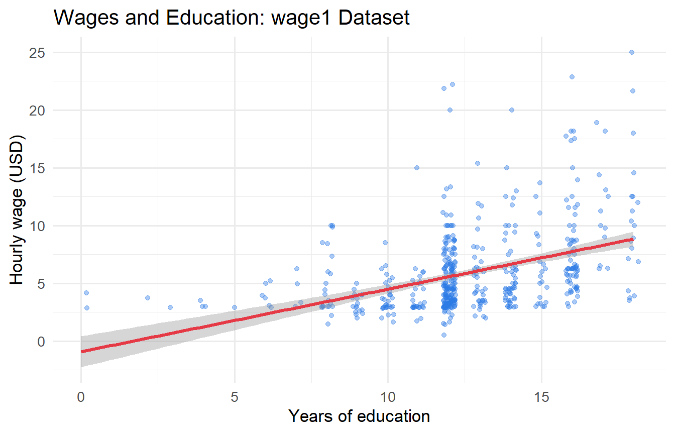
#| fig-cap: "Hourly wages and years of education. Line = OLS fit with 95% confidence band."
ggplot(wage1, aes(x = educ, y = wage)) +
  geom_jitter(alpha = 0.4, width = 0.2, colour = "#2c7be5") +
  geom_smooth(method = "lm", colour = "#e63946", linewidth = 1.2, se = TRUE) +
  labs(x = "Years of education", y = "Hourly wage (USD)",
       title = "Wages and Education: wage1 Dataset")
```
### Fitting and Reading OLS Output
```{r}
#| label: slr-wage
fit_slr <- lm(wage ~ educ, data = wage1)
tidy(fit_slr, conf.int = TRUE)
```
```{r}
#| label: slr-wage-glance
glance(fit_slr) |> select(r.squared, adj.r.squared, sigma, nobs)
```
- **Intercept** $(\hat{\beta}_0 \approx `r round(coef(fit_slr)[1], 2)`)$: Predicted wage with zero years of education. Interpret with caution — this is outside the support of the data.
- **Slope** $(\hat{\beta}_1 \approx `r round(coef(fit_slr)[2], 2)`)$: Each additional year of schooling is associated with \$`r round(coef(fit_slr)[2], 2)` more per hour on average.
- **$R^2 \approx `r round(glance(fit_slr)$r.squared, 3)`$**: Education explains `r round(glance(fit_slr)$r.squared * 100, 1)`% of the variation in wages. A low $R^2$ here is not a problem; many factors other than education affect wages.
- **SER $\approx `r round(glance(fit_slr)$sigma, 2)`$**: Residuals are on average \$`r round(glance(fit_slr)$sigma, 2)` away from the fitted line.
### Manual Computation and Verification
```{r}
#| label: ols-manual
wage1 |>
  summarise(
    x_bar  = mean(educ),
    y_bar  = mean(wage),
    cov_xy = sum((educ - mean(educ)) * (wage - mean(wage))),
    var_x  = sum((educ - mean(educ))^2),
    beta_1 = cov_xy / var_x,
    beta_0 = y_bar - beta_1 * x_bar
  )
```
```{r}
#| label: ols-matrix
# Matrix form: beta_hat = (X'X)^{-1} X'y
y_vec <- wage1$wage
X_mat <- cbind(1, wage1$educ)

beta_matrix <- solve(t(X_mat) %*% X_mat) %*% (t(X_mat) %*% y_vec)
round(beta_matrix, 4)   # identical to lm() output
```
All three routes — closed-form formula, `lm()`, and matrix algebra — agree exactly.
### Verifying the Decomposition
```{r}
#| label: r-squared-manual
aug <- augment(fit_slr)

SST <- sum((aug$wage        - mean(aug$wage))^2)
SSE <- sum((aug$.fitted     - mean(aug$wage))^2)
SSR <- sum( aug$.resid^2)

cat("SST:", round(SST, 2), "\n")
cat("SSE:", round(SSE, 2), "\n")
cat("SSR:", round(SSR, 2), "\n")
cat("SST == SSE + SSR:", isTRUE(all.equal(SST, SSE + SSR)), "\n")
cat("R-squared:", round(SSE / SST, 4), "\n")
```
### Residual Diagnostics
```{r}
#| label: fig-residuals
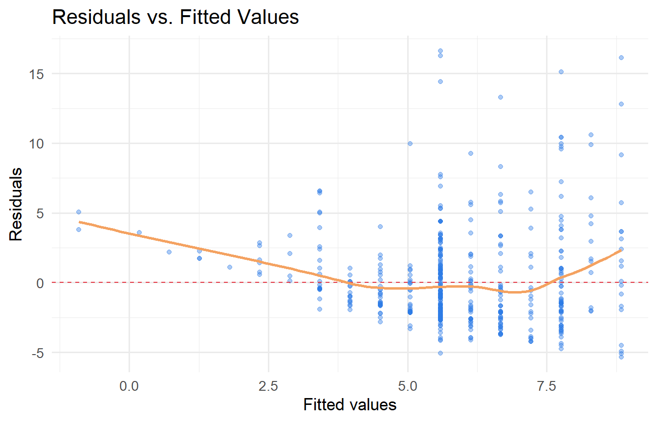
#| fig-cap: "Residuals versus fitted values. A pattern here signals model misspecification."
aug |>
  ggplot(aes(.fitted, .resid)) +
  geom_point(alpha = 0.4, colour = "#2c7be5") +
  geom_hline(yintercept = 0, linetype = "dashed", colour = "#e63946") +
  geom_smooth(se = FALSE, colour = "#f4a261", linewidth = 1) +
  labs(x = "Fitted values", y = "Residuals",
       title = "Residuals vs. Fitted Values")
```
The spread of residuals increases slightly with fitted values — a hint of heteroskedasticity that we return to in Chapter 9.
---
## Multiple Regression: A Preview
With two regressors the PRF becomes $E[y \mid x_1, x_2] = \beta_0 + \beta_1 x_1 + \beta_2 x_2$.
The **partial effect** of $x_1$ holding $x_2$ fixed is $\Delta \hat{y} = \hat{\beta}_1 \Delta x_1$. That is, $\hat{\beta}_1$ estimates the effect of $x_1$ on $y$ **after removing the variation in $y$ attributable to $x_2$**.
```{r}
#| label: mlr-preview
data("wage2", package = "wooldridge")

fit_iq <- lm(wage ~ educ + IQ, data = wage2)

modelsummary(
  list("SLR (educ only)" = lm(wage ~ educ, data = wage2),
       "MLR (educ + IQ)"  = fit_iq),
  stars   = TRUE,
  gof_map = c("nobs", "r.squared"),
  title   = "Education and IQ as Determinants of Wages"
)
```
Including IQ as a control reduces the education coefficient substantially. The SLR coefficient was picking up intelligence: smart people both acquire more education **and** earn more. Once IQ is held constant, the estimated return to education is smaller and represents a more credible partial effect.
---
## Tutorials
**Tutorial 3.1** Using `wooldridge::wage1`:
a. Regress `wage` on `exper` (experience). Report and interpret $\hat{\beta}_0$ and $\hat{\beta}_1$.
b. What is the predicted wage for someone with 10 years of experience?
c. What is $R^2$? Is it higher or lower than the education regression? What does this tell you?
::: {.callout-tip collapse="true"}
## Solution
```{r}
#| label: ex3-1
fit_exper <- lm(wage ~ exper, data = wage1)
tidy(fit_exper, conf.int = TRUE)
predict(fit_exper, newdata = tibble(exper = 10))
glance(fit_exper) |> select(r.squared)
```
- $\hat{\beta}_0 \approx `r round(coef(fit_exper)[1], 2)`$: predicted wage with zero experience.
- $\hat{\beta}_1 \approx `r round(coef(fit_exper)[2], 3)`$: each additional year of experience adds approximately \$`r round(coef(fit_exper)[2], 3)` to the hourly wage.
- Predicted wage at 10 years: \$`r round(predict(fit_exper, newdata = tibble(exper = 10)), 2)`.
- $R^2$ from experience: `r round(glance(fit_exper)$r.squared, 3)`, lower than the education regression (`r round(glance(fit_slr)$r.squared, 3)`). Education explains more cross-sectional variation in wages than experience does.
:::
---
**Tutorial 3.2** Verify the geometry of OLS numerically. Use any three-observation dataset of your choice (or the house example from Section 5).
a. Construct $\mathbf{y}$, $\mathbf{X}$, and compute $\hat{\boldsymbol{\beta}} = (\mathbf{X'X})^{-1}\mathbf{X'y}$ by hand in R.
b. Verify that $\mathbf{X'}\hat{\mathbf{u}} = \mathbf{0}$.
c. Compute $\mathbf{P}_X$ and $\mathbf{M}_X$. Check that they are idempotent and orthogonal to each other.
d. Verify Pythagoras: $\|\tilde{\mathbf{y}}\|^2 = \|\tilde{\hat{\mathbf{y}}}\|^2 + \|\hat{\mathbf{u}}\|^2$.
::: {.callout-tip collapse="true"}
## Solution
```{r}
#| label: ex3-2
y <- c(10, 4, 6)
X <- cbind(1, c(4, 1, 1))

# (a) OLS via matrix formula
beta_hat <- solve(t(X) %*% X) %*% (t(X) %*% y)
y_hat    <- X %*% beta_hat
u_hat    <- y - y_hat

cat("beta_hat:", round(beta_hat, 4), "\n")
# (b) Orthogonality
cat("X'u_hat:", round(t(X) %*% u_hat, 10), "\n")
# (c) Projection matrices
n  <- length(y)
P  <- X %*% solve(t(X) %*% X) %*% t(X)
M  <- diag(n) - P
cat("Idempotent P:  ", max(abs(P %*% P - P)) < 1e-10, "\n")
cat("Idempotent M: ", max(abs(M %*% M - M)) < 1e-10, "\n")
cat("P orthog. to M:", max(abs(P %*% M)) < 1e-10, "\n")
# (d) Pythagorean decomposition
ybar  <- mean(y)
SST   <- sum((y     - ybar)^2)
SSE   <- sum((y_hat - ybar)^2)
SSR   <- sum(u_hat^2)
cat("SST:", round(SST, 4), " SSE:", round(SSE, 4), " SSR:", round(SSR, 4), "\n")
cat("SST == SSE + SSR:", isTRUE(all.equal(SST, SSE + SSR)), "\n")
```
:::
---
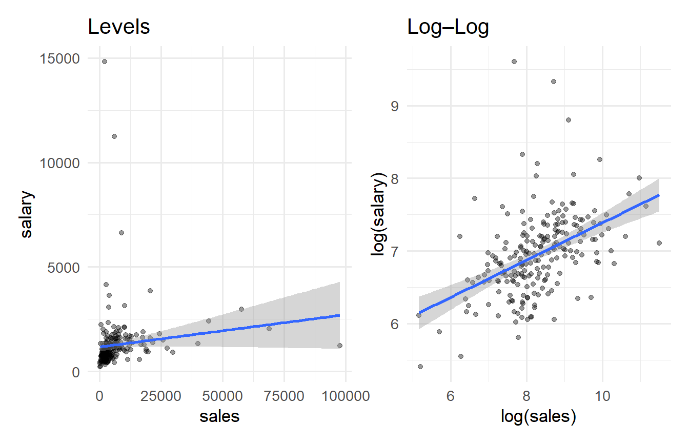
**Tutorial 3.3** Using `wooldridge::ceosal1`, regress CEO salary (`salary`) on firm sales (`sales`).
a. Interpret the slope coefficient.
b. Does the linear fit look appropriate? (Plot salary vs. sales.)
c. Regress `log(salary)` on `log(sales)`. How does the slope interpretation change?
::: {.callout-tip collapse="true"}
## Solution
```{r}
#| label: ex3-3
#| fig-cap: "CEO salary on sales: levels vs. log–log."
data("ceosal1", package = "wooldridge")

fit_levels <- lm(salary ~ sales, data = ceosal1)
fit_logs   <- lm(log(salary) ~ log(sales), data = ceosal1)

p1 <- ggplot(ceosal1, aes(sales, salary)) +
  geom_point(alpha = 0.4) + geom_smooth(method = "lm") +
  labs(title = "Levels")

p2 <- ggplot(ceosal1, aes(log(sales), log(salary))) +
  geom_point(alpha = 0.4) + geom_smooth(method = "lm") +
  labs(title = "Log–Log")

p1 + p2
modelsummary(list("Levels" = fit_levels, "Log-Log" = fit_logs),
             stars = TRUE, gof_map = c("nobs", "r.squared"))
```
In the log–log model, $\hat{\beta}_1$ is an **elasticity**: a 1% increase in sales is associated with approximately `r round(coef(fit_logs)[2], 3)`% increase in salary. The log–log specification fits considerably better because both variables are right-skewed; the levels regression is distorted by outliers.
:::