---
title: "Chapter 7: Functional Form, Dummies, and Interactions"
subtitle: "Non-linearities, qualitative variables, and interaction effects"
---
```{r}
#| label: setup
#| include: false
library(tidyverse)
library(broom)
library(modelsummary)
library(car)
library(patchwork)
library(wooldridge)
theme_set(theme_minimal(base_size = 13))
options(digits = 4, scipen = 999)
data("wage1", package = "wooldridge")
```
::: {.callout-note}
## Learning Objectives
By the end of this chapter you will be able to:
- Interpret exact percentage changes from log-level models via $e^{\hat{\beta}} - 1$
- Incorporate quadratic and polynomial terms and compute marginal effects
- Explain the dummy variable trap using the $\mathbf{X}$-matrix rank argument
- Include multi-category dummy variables and interpret pairwise differences invariantly across base category choices
- Construct and interpret interaction terms between a dummy and a continuous variable
- Conduct the Chow test for structural breaks, both manually and via `linearHypothesis()`
:::
---
## Log Functional Forms: Exact Interpretation
Chapter 6 introduced the log approximation $100\Delta\ln(z) \approx \%\Delta z$. For log-level and log-log models, the **exact** interpretation matters when coefficients are large.
### Exact Percentage Change in Log-Level Models
In the model $\ln y = \beta_0 + \beta_1 x + u$, a one-unit increase in $x$ changes $\ln y$ by $\beta_1$. The **exact** percentage change in $y$ is:
$$y_{after} = e^{\beta_0 + \beta_1(x+1) + u} = e^{\beta_1} \cdot e^{\beta_0 + \beta_1 x + u} = e^{\beta_1} \cdot y_{before}$$
Therefore:
$$\frac{y_{after} - y_{before}}{y_{before}} = e^{\beta_1} - 1$$
In percentage terms: $\% \Delta y = 100(e^{\hat{\beta}_1} - 1)$.
The approximation $100\hat{\beta}_1$ equals the first-order Taylor expansion of $100(e^{\hat{\beta}_1} - 1)$ around $\hat{\beta}_1 = 0$. For $|\hat{\beta}_1| < 0.1$, the error is less than 5% of the coefficient. For larger values, always report the exact figure.
```{r}
#| label: exact-pct-change
wage1 <- wage1 |> mutate(lwage = log(wage))
fit_log <- lm(lwage ~ educ + exper + I(exper^2) + tenure + female, data = wage1)

b_female <- coef(fit_log)["female"]
cat("Coefficient on female:", round(b_female, 4), "\n")
cat("Approximate % change: ", round(100 * b_female, 2), "%\n")
cat("Exact % change: ", round(100 * (exp(b_female) - 1), 2), "%\n")
```
The approximate and exact figures differ meaningfully for `female` because the coefficient is not small. The **exact** figure should be reported.
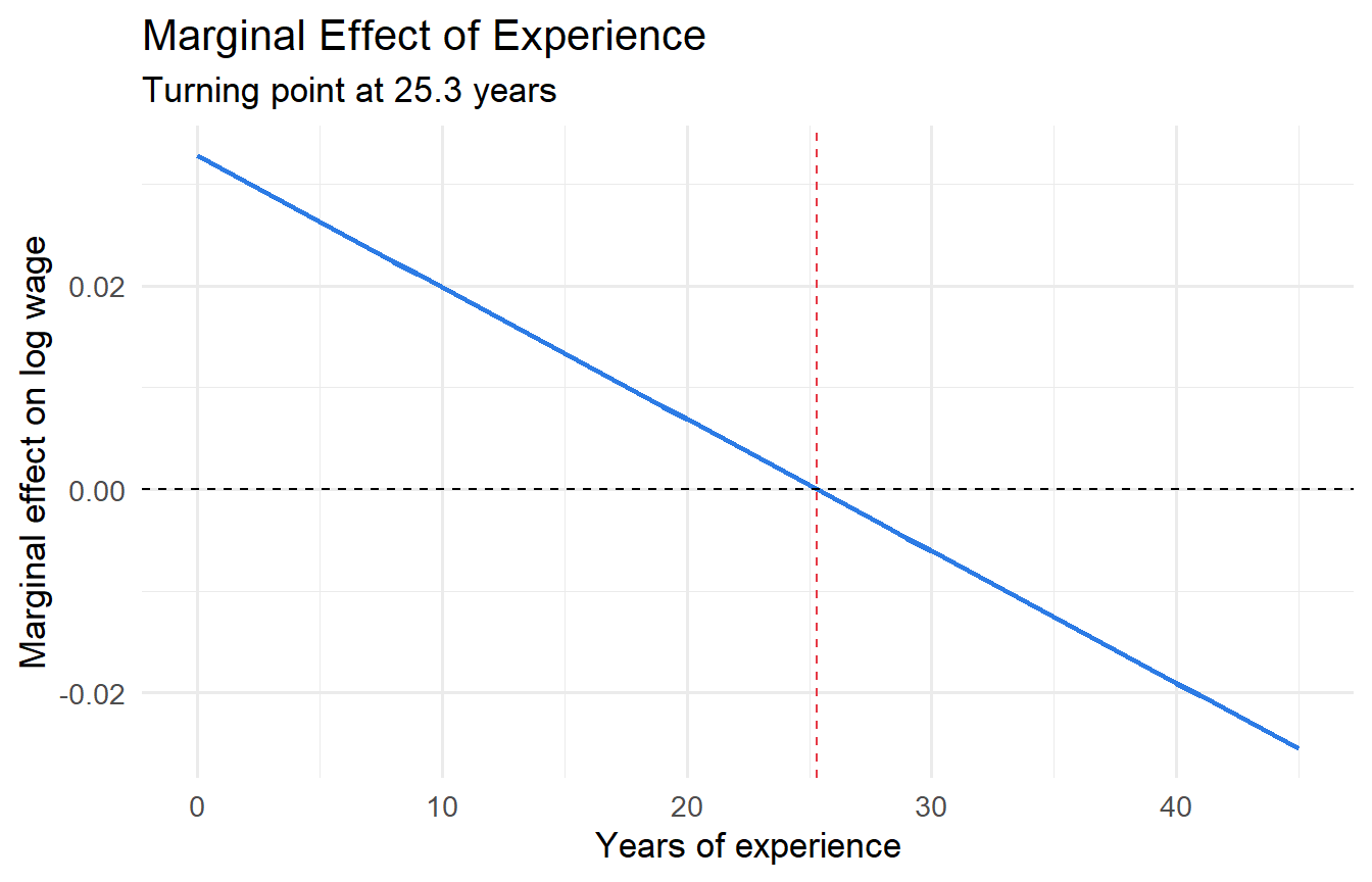
### Quadratic Terms and Marginal Effects
When the effect of $x$ on $y$ is non-linear:
$$y = \beta_0 + \beta_1 x + \beta_2 x^2 + u$$
The **marginal effect** is $\partial y / \partial x = \beta_1 + 2\beta_2 x$ — it varies with $x$. When $\beta_2 < 0$, the relationship is concave with a maximum (turning point) at:
$$x^* = -\frac{\beta_1}{2\beta_2}$$
```{r}
#| label: quadratic-exper
#| fig-cap: "Diminishing returns to experience: marginal effect crosses zero at the turning point."
b_exper  <- coef(fit_log)["exper"]
b_exper2 <- coef(fit_log)["I(exper^2)"]
tp <- -b_exper / (2 * b_exper2)

tibble(exper = 0:45) |>
  mutate(marginal = b_exper + 2 * b_exper2 * exper) |>
  ggplot(aes(exper, marginal)) +
  geom_line(colour = "#2c7be5", linewidth = 1) +
  geom_hline(yintercept = 0, linetype = "dashed") +
  geom_vline(xintercept = tp, colour = "#e63946", linetype = "dashed") +
  labs(x = "Years of experience", y = "Marginal effect on log wage",
       title = "Marginal Effect of Experience",
       subtitle = paste0("Turning point at ", round(tp, 1), " years"))
```
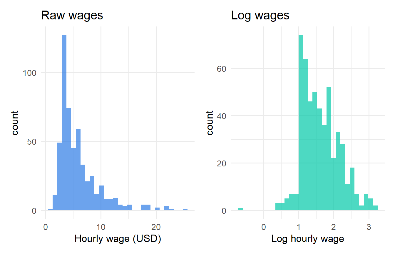
```{r}
#| label: fig-log-wage
#| fig-cap: "Raw wages are right-skewed; log wages are approximately symmetric."
p1 <- ggplot(wage1, aes(wage)) +
  geom_histogram(bins = 30, fill = "#2c7be5", alpha = 0.7) +
  labs(x = "Hourly wage (USD)", title = "Raw wages")
p2 <- ggplot(wage1, aes(lwage)) +
  geom_histogram(bins = 30, fill = "#00c9a7", alpha = 0.7) +
  labs(x = "Log hourly wage", title = "Log wages")
p1 + p2
```
---
## Dummy Variables
A **dummy variable** (indicator variable) takes the value 1 if a condition is met and 0 otherwise:
$$D_i = \begin{cases} 1 & \text{if condition is true} \\ 0 & \text{otherwise} \end{cases}$$
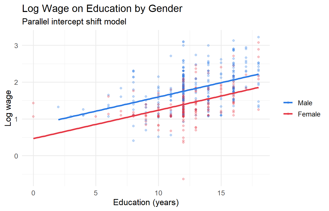
### Intercept Shift
Including a dummy causes a **parallel shift** in the regression line — the slope is the same for both groups but the intercept differs by $\delta$:
$$\ln(wage_i) = \beta_0 + \beta_1 educ_i + \delta \cdot female_i + u_i$$
$\delta$ measures the expected difference in log wages between women and men at any education level, all else equal.
```{r}
#| label: fig-dummy-shift
#| fig-cap: "Parallel regression lines: separate intercepts by gender, same slopes."
ggplot(wage1, aes(educ, lwage, colour = factor(female))) +
  geom_point(alpha = 0.3) +
  geom_smooth(method = "lm", se = FALSE, linewidth = 1.2) +
  scale_colour_manual(values = c("#2c7be5","#e63946"),
                      labels = c("Male","Female")) +
  labs(x = "Education (years)", y = "Log wage",
       colour = NULL, title = "Log Wage on Education by Gender",
       subtitle = "Parallel intercept shift model")
```
### The Dummy Variable Trap: A Rank Argument
For a categorical variable with $m$ categories, include **exactly** $m - 1$ dummies. Including all $m$ creates **perfect multicollinearity** — a structural failure, not a data problem.
**Proof.** Suppose we have two regions (A and B) and include both $D_A$ and $D_B$ plus an intercept. The design matrix has columns:
$$\mathbf{X} = \begin{bmatrix} 1 & D_{A1} & D_{B1} \\ 1 & D_{A2} & D_{B2} \\ \vdots & \vdots & \vdots \end{bmatrix}$$
Since every observation is in exactly one region, $D_{Ai} + D_{Bi} = 1$ for all $i$. Therefore the intercept column equals the sum of the two dummy columns:
$$\mathbf{1} = \mathbf{D}_A + \mathbf{D}_B$$
This is an exact linear dependency. $\text{rank}(\mathbf{X}) < k + 1$, so $\mathbf{X}'\mathbf{X}$ is singular and $(\mathbf{X}'\mathbf{X})^{-1}$ does not exist. OLS has no unique solution — there are infinitely many coefficient vectors that minimise SSR equally. The software either drops a dummy automatically or reports an error. $\blacksquare$
More generally, for $m$ categories with dummies $D_1, \ldots, D_m$: $\sum_{j=1}^m D_j = \mathbf{1}$, so any $m$ of the $m+1$ columns $\{\mathbf{1}, D_1, \ldots, D_m\}$ are linearly dependent.
### Multi-Category Dummies and Invariance of Pairwise Differences
```{r}
#| label: multi-category
wage1 <- wage1 |>
  mutate(region = case_when(
    northcen == 1 ~ "North Central",
    south    == 1 ~ "South",
    west     == 1 ~ "West",
    TRUE          ~ "Northeast"
  ) |> factor(levels = c("Northeast","North Central","South","West")))

fit_r_NE <- lm(lwage ~ educ + exper + tenure + female + region, data = wage1)
tidy(fit_r_NE) |> dplyr::filter(str_detect(term, "region"))
```
Each coefficient is the difference in conditional mean log wages relative to the **base category** (Northeast). A natural concern: does changing the base category change the substantive conclusions?
**Pairwise differences are invariant to the choice of base category.**
With Northeast as base:
$$\hat{\mu}_{South} - \hat{\mu}_{NE} = \hat{\delta}_{South}, \quad \hat{\mu}_{West} - \hat{\mu}_{NE} = \hat{\delta}_{West}$$
The South–West difference is $\hat{\delta}_{South} - \hat{\delta}_{West}$. If we re-estimate with West as base, the South coefficient becomes $\hat{\mu}_{South} - \hat{\mu}_{West}$, which equals $\hat{\delta}_{South} - \hat{\delta}_{West}$ — the same number. Only the **pairwise differences** (not the individual coefficients) have interpretation independent of the base.
```{r}
#| label: base-invariance
# Re-estimate with South as base
wage1_s <- wage1 |>
  mutate(region_s = relevel(region, ref = "South"))

fit_r_S <- lm(lwage ~ educ + exper + tenure + female + region_s, data = wage1_s)

# West - North Central difference: should be the same regardless of base
d_NE <- tidy(fit_r_NE) |> dplyr::filter(term == "regionNorth Central") |> dplyr::pull(estimate)
d_W  <- tidy(fit_r_NE) |> dplyr::filter(term == "regionWest") |> dplyr::pull(estimate)
d_W_fromS <- tidy(fit_r_S) |> dplyr::filter(term == "region_sWest") |> dplyr::pull(estimate)
d_NC_fromS <- tidy(fit_r_S) |> dplyr::filter(term == "region_sNorth Central") |> dplyr::pull(estimate)

cat("West - North Central (NE base):", round(d_W - d_NE, 6), "\n")
cat("West - North Central (S base):", round(d_W_fromS - d_NC_fromS, 6), "\n")
```
The pairwise difference is identical to machine precision, confirming the invariance.
---
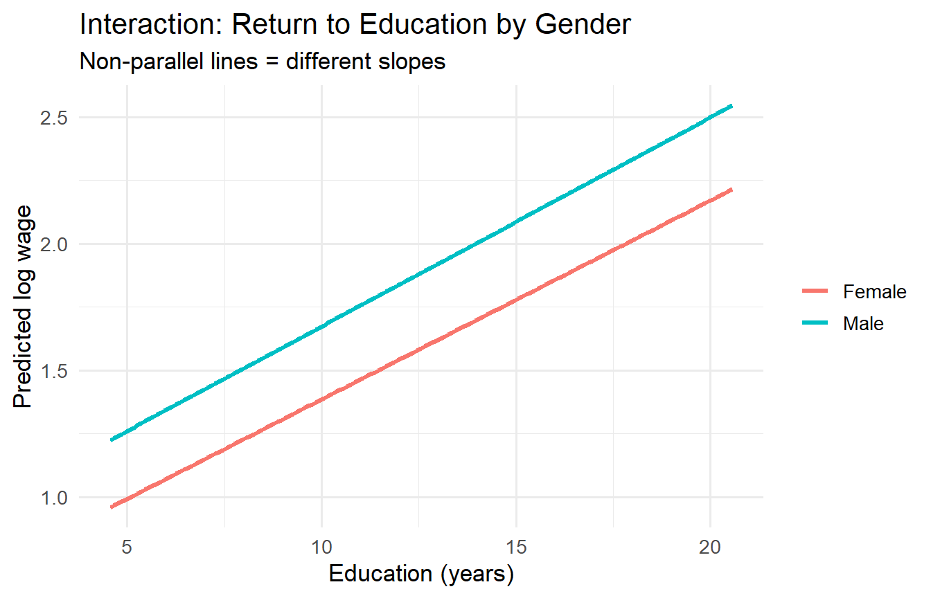
## Interaction Terms
An **interaction term** $x \times D$ allows the **slope** on $x$ to differ across groups:
$$\ln(wage_i) = \beta_0 + \beta_1 educ_i + \delta_0 female_i + \delta_1 (educ_i \times female_i) + u_i$$
- For men ($D=0$): $E[\ln wage \mid educ, D=0] = \beta_0 + \beta_1 \, educ$
- For women ($D=1$): $E[\ln wage \mid educ, D=1] = (\beta_0 + \delta_0) + (\beta_1 + \delta_1) \, educ$
$\delta_1$ captures the **differential return to education** for women relative to men.
### Multicollinearity in Interaction Models
A frequent puzzle: after including `female` and `female × educ`, the correlation between them is high. This is not a bug — it is a genuine mechanical correlation:
```{r}
#| label: interaction-collinearity
wage1 <- wage1 |> mutate(female_x_educ = female * educ)
cat("Correlation between female and female×educ:",
    round(cor(wage1$female, wage1$female_x_educ), 3), "\n")
```
High correlation between `female` and `female × educ` is expected: the interaction is literally a function of one of the main effects. This **does not** invalidate the model or the $t$-test on $\delta_1$. It inflates individual standard errors but the joint test (F-test for both `female` and `female × educ`) remains valid. **Centring** the continuous variable ($educ^* = educ - \bar{educ}$) reduces this correlation substantially without changing the substantive results.
```{r}
#| label: interaction-centred
wage1 <- wage1 |> mutate(educ_c = educ - mean(educ))
fit_int_c <- lm(lwage ~ educ_c * female + exper + I(exper^2) + tenure, data = wage1)
cat("Correlation after centring:",
    round(cor(wage1$female, wage1$female * wage1$educ_c), 3), "\n")
tidy(fit_int_c, conf.int = TRUE) |>
  dplyr::filter(term %in% c("educ_c", "female", "educ_c:female"))
```
After centring, the `female` coefficient is now the gender gap **at the mean education level** (not at $educ = 0$, which is extrapolation).
```{r}
#| label: fig-interaction
#| fig-cap: "Return to education is steeper for men than women (interaction model)."
newdata <- expand_grid(
  educ_c = seq(-8, 8, 0.1),
  female = 0:1,
  exper  = mean(wage1$exper),
  tenure = mean(wage1$tenure)
)
newdata |>
  mutate(
    pred   = predict(fit_int_c, newdata = newdata),
    gender = if_else(female == 1, "Female", "Male"),
    educ   = educ_c + mean(wage1$educ)
  ) |>
  ggplot(aes(educ, pred, colour = gender)) +
  geom_line(linewidth = 1.2) +
  labs(x = "Education (years)", y = "Predicted log wage", colour = NULL,
       title = "Interaction: Return to Education by Gender",
       subtitle = "Non-parallel lines = different slopes")
```
---
## The Chow Test for Structural Breaks
A **Chow test** asks whether the **entire** regression relationship — all slopes and the intercept — differs across two groups or time periods. It is an $F$-test that compares:
- **Restricted**: single regression for both groups (pooled, with possible intercept shift)
- **Unrestricted**: separate regressions for each group
### Manual Computation
Let $SSR_R$ = SSR from the restricted (pooled) model, $SSR_{UR}$ = $SSR_M + SSR_F$ (sum of SSRs from separate male and female regressions), $q$ = number of restrictions (the number of slope coefficients tested), $k$ = number of regressors in each group model.
$$F = \frac{(SSR_R - SSR_{UR})/q}{SSR_{UR}/(n - 2(k+1))} \sim F(q,\, n - 2(k+1))$$
```{r}
#| label: chow-test-manual
# Male and female subsets
wage_m <- wage1 |> dplyr::filter(female == 0)
wage_f <- wage1 |> dplyr::filter(female == 1)

# Regressors in each model: educ, exper, exper^2, tenure (k=4, so k+1=5 params)
formula_chow <- lwage ~ educ + exper + I(exper^2) + tenure

fit_m   <- lm(formula_chow, data = wage_m)
fit_f   <- lm(formula_chow, data = wage_f)
fit_r   <- lm(lwage ~ educ + exper + I(exper^2) + tenure + female, data = wage1)

SSR_UR <- sum(resid(fit_m)^2) + sum(resid(fit_f)^2)
SSR_R  <- sum(resid(fit_r)^2)
n      <- nrow(wage1)
k1     <- length(coef(fit_m))   # number of params in each group model
q      <- k1 - 1                # slopes only (the intercept is already allowed to differ)

F_chow <- ((SSR_R - SSR_UR) / q) / (SSR_UR / (n - 2 * k1))
p_chow <- pf(F_chow, q, n - 2 * k1, lower.tail = FALSE)

cat("SSR restricted (with female dummy):", round(SSR_R,  2), "\n")
cat("SSR unrestricted (male + female): ", round(SSR_UR, 2), "\n")
cat("F-statistic:", round(F_chow, 4), "\n")
cat("p-value: ", round(p_chow, 4), "\n")
```
```{r}
#| label: chow-test-verify
# Verify via linearHypothesis: test all slope interactions jointly
fit_full_int <- lm(lwage ~ (educ + exper + I(exper^2) + tenure) * female, data = wage1)
linearHypothesis(fit_full_int,
                 c("educ:female = 0", "exper:female = 0",
                   "I(exper^2):female = 0", "tenure:female = 0"))
```
A significant $F$ rejects the null that all slope coefficients are equal across men and women.
### Structural Break in Time Series
The Chow test also applies to time series at a known break date. Let $D_t^{post}$ be a post-break dummy. An equivalent implementation: include all interactions of regressors with $D_t^{post}$ and test them jointly.
```{r}
#| label: structural-break
data("intdef", package = "wooldridge")  # interest rate & inflation, US 1948-2003

# Mark post-1979 (Volcker shock) as a potential structural break
intdef <- intdef |>
  mutate(post79 = as.integer(year >= 1979))

fit_pre  <- lm(i3 ~ inf + def, data = dplyr::filter(intdef, post79 == 0))
fit_post <- lm(i3 ~ inf + def, data = dplyr::filter(intdef, post79 == 1))
fit_pool <- lm(i3 ~ inf + def + post79, data = intdef)
fit_brk  <- lm(i3 ~ (inf + def) * post79, data = intdef)

SSR_UR_ts <- sum(resid(fit_pre)^2) + sum(resid(fit_post)^2)
SSR_R_ts  <- sum(resid(fit_pool)^2)
n_ts <- nrow(intdef); k_ts <- 3
F_ts <- ((SSR_R_ts - SSR_UR_ts) / 2) / (SSR_UR_ts / (n_ts - 2 * k_ts))
cat("Chow F-statistic for 1979 break:", round(F_ts, 3), "\n")
cat("p-value:", round(pf(F_ts, 2, n_ts - 2*k_ts, lower.tail = FALSE), 4), "\n")
```
A significant result suggests the relationship between interest rates, inflation, and the deficit changed structurally around the Volcker disinflation.
---
## Tutorials
**Tutorial 7.1**
Using `wooldridge::wage1`, estimate the log wage model with quadratic experience and the `female` dummy. Compute the experience level at which the wage-experience profile peaks. Report the **exact** (not approximate) percentage wage gap for women.
::: {.callout-tip collapse="true"}
## Solution
```{r}
#| label: ex7-1
fit_q <- lm(lwage ~ educ + exper + I(exper^2) + tenure + female, data = wage1)
b1    <- coef(fit_q)["exper"]
b2    <- coef(fit_q)["I(exper^2)"]
tp    <- -b1 / (2 * b2)

d_fem    <- coef(fit_q)["female"]
exact_pct <- 100 * (exp(d_fem) - 1)

cat("Turning point:", round(tp, 1), "years\n")
cat("Data range: ", min(wage1$exper), "to", max(wage1$exper), "\n\n")
cat("Approx gender gap:", round(100*d_fem, 2), "%\n")
cat("Exact gender gap: ", round(exact_pct, 2), "%\n")
```
:::
**Tutorial 7.2**
Show the dummy variable trap in practice. Attempt to include dummies for all four regions (`Northeast`, `North Central`, `South`, `West`) plus an intercept. What does R do? Explain algebraically why the model is not identified.
::: {.callout-tip collapse="true"}
## Solution
```{r}
#| label: ex7-2
# R silently drops one dummy due to perfect collinearity
wage1_trap <- wage1 |>
  mutate(
    d_NE = as.integer(region == "Northeast"),
    d_NC = as.integer(region == "North Central"),
    d_S  = as.integer(region == "South"),
    d_W  = as.integer(region == "West")
  )

fit_trap <- lm(lwage ~ educ + d_NE + d_NC + d_S + d_W, data = wage1_trap)
cat("Coefficients returned (note NA):\n")
print(coef(fit_trap))
# Verify the linear dependency: sum of all dummies = 1
with(wage1_trap, all(d_NE + d_NC + d_S + d_W == 1))
```
R drops `d_W` (the last dummy) and returns `NA` for it — a sign of the trap. The algebraic reason: $\mathbf{D}_{NE} + \mathbf{D}_{NC} + \mathbf{D}_S + \mathbf{D}_W = \mathbf{1}$ (the intercept column), so the columns of $\mathbf{X}$ are linearly dependent and $\mathbf{X}'\mathbf{X}$ is singular.
:::
**Tutorial 7.3**
Conduct a Chow test for whether the wage regression (`lwage ~ educ + exper + tenure`) has the same slope coefficients for `nonwhite` vs. white workers. Compute the F-statistic by hand (using separate SSRs) and verify with `linearHypothesis()`.
::: {.callout-tip collapse="true"}
## Solution
```{r}
#| label: ex7-3
formula_w <- lwage ~ educ + exper + tenure

fit_white    <- lm(formula_w, data = dplyr::filter(wage1, nonwhite == 0))
fit_nonwhite <- lm(formula_w, data = dplyr::filter(wage1, nonwhite == 1))
fit_pool_w   <- lm(lwage ~ educ + exper + tenure + nonwhite, data = wage1)

SSR_UR2 <- sum(resid(fit_white)^2) + sum(resid(fit_nonwhite)^2)
SSR_R2  <- sum(resid(fit_pool_w)^2)
n2      <- nrow(wage1)
k2      <- length(coef(fit_white))
q2      <- k2 - 1

F2   <- ((SSR_R2 - SSR_UR2) / q2) / (SSR_UR2 / (n2 - 2 * k2))
p2   <- pf(F2, q2, n2 - 2*k2, lower.tail = FALSE)
cat("Chow F-statistic:", round(F2, 4), "  p-value:", round(p2, 4), "\n")
# Verify
fit_int_race <- lm(lwage ~ (educ + exper + tenure) * nonwhite, data = wage1)
linearHypothesis(fit_int_race,
                 c("educ:nonwhite = 0", "exper:nonwhite = 0", "tenure:nonwhite = 0"))
```
:::