---
title: "Chapter 8: Large Sample Properties"
subtitle: "Consistency, the Law of Large Numbers, and asymptotic normality"
---
```{r}
#| label: setup
#| include: false
library(tidyverse)
library(broom)
library(patchwork)
theme_set(theme_minimal(base_size = 13))
options(digits = 4, scipen = 999)
set.seed(2024)
```
::: {.callout-note}
## Learning Objectives
By the end of this chapter you will be able to:
- State and apply the Weak Law of Large Numbers (WLLN) and the Central Limit Theorem (CLT)
- Apply the Continuous Mapping Theorem (CMT) and Slutsky's theorem to derive limiting distributions
- Derive the consistency of OLS in both scalar and matrix form
- Derive the asymptotic normality of OLS from the CLT
- Explain why large-sample theory validates inference without normality of errors
- Demonstrate CLT convergence and OLS consistency via simulation
:::
---
## Why Large-Sample Theory?
The finite-sample results from Chapters 4–5 relied on **MLR.6** — normally distributed errors. In practice, errors are rarely normal. How can we justify using $t$- and $F$-distributions for inference?
The answer is **asymptotic (large-sample) theory**: as $n \to \infty$, OLS estimators behave like normal random variables **regardless of the error distribution**. This is the Central Limit Theorem at work.
Large-sample theory also tells us:
- OLS is consistent under conditions weaker than unbiasedness requires
- When MLR.5 (homoskedasticity) fails, the standard SE formula is wrong — we need **robust** standard errors
- For time-series data with serial correlation, we need **HAC** standard errors
Both of these fixes (Chapters 9–10) are justified by asymptotic theory.
---
## Convergence Concepts
### Convergence in Probability and Consistency
A sequence of random variables $\{W_n\}$ **converges in probability** to a constant $c$ if:
$$\forall \varepsilon > 0: \quad \lim_{n \to \infty} P(|W_n - c| > \varepsilon) = 0$$
Written $W_n \xrightarrow{p} c$ or $\text{plim}_{n \to \infty} W_n = c$. An estimator $\hat{\theta}_n$ is **consistent** for $\theta$ if $\hat{\theta}_n \xrightarrow{p} \theta$.
### Convergence in Distribution
$\{W_n\}$ **converges in distribution** to a random variable $W$ if for every continuity point $w$ of the CDF of $W$:
$$\lim_{n \to \infty} P(W_n \leq w) = P(W \leq w)$$
Written $W_n \xrightarrow{d} W$. This is weaker than convergence in probability: if $W_n \xrightarrow{p} c$, then $W_n \xrightarrow{d} c$, but not vice versa.
### Two Essential Results
::: {.callout-note}
## Continuous Mapping Theorem (CMT)
If $W_n \xrightarrow{p} c$ and $g(\cdot)$ is continuous at $c$, then $g(W_n) \xrightarrow{p} g(c)$.
Implication: $\text{plim}(A_n^{-1}) = [\text{plim}(A_n)]^{-1}$ if $\text{plim}(A_n)$ is invertible. This is what allows us to carry the matrix inverse through the probability limit.
:::
::: {.callout-note}
## Slutsky's Theorem
If $A_n \xrightarrow{d} A$ and $B_n \xrightarrow{p} c$ (a constant), then:
$$A_n + B_n \xrightarrow{d} A + c, \qquad A_n B_n \xrightarrow{d} cA, \qquad A_n / B_n \xrightarrow{d} A/c$$
Implication: we can substitute a consistent estimator for an unknown population parameter in a limiting distribution without changing the limit.
:::
---
## The Law of Large Numbers
::: {.callout-note}
## Weak Law of Large Numbers (WLLN)
If $X_1, X_2, \ldots$ are i.i.d. with $E[X_i] = \mu < \infty$ and $\text{Var}(X_i) < \infty$, then:
$$\bar{X}_n = \frac{1}{n}\sum_{i=1}^n X_i \xrightarrow{p} \mu$$
:::
**Proof sketch.** By Chebyshev's inequality:
$$P(|\bar{X}_n - \mu| > \varepsilon) \leq \frac{\text{Var}(\bar{X}_n)}{\varepsilon^2} = \frac{\sigma^2}{n\varepsilon^2} \to 0 \text{ as } n \to \infty. \qquad \blacksquare$$
The *Strong* LLN (Kolmogorov) guarantees almost-sure convergence ($P(\lim \bar{X}_n = \mu) = 1$) under the same conditions; the WLLN is sufficient for econometrics.
```{r}
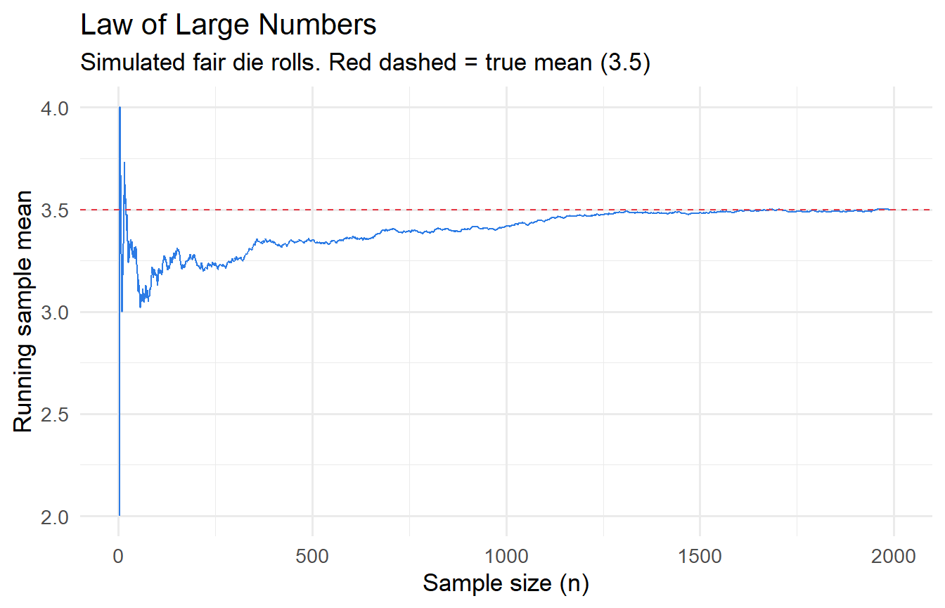
#| label: fig-lln
#| fig-cap: "LLN: sample means converge to the population mean as n grows."
true_mu <- 3.5
n_max   <- 2000

tibble(
  n        = 1:n_max,
  cum_mean = cumsum(sample(1:6, n_max, replace = TRUE)) / 1:n_max
) |>
  ggplot(aes(n, cum_mean)) +
  geom_line(colour = "#2c7be5") +
  geom_hline(yintercept = true_mu, colour = "#e63946", linetype = "dashed") +
  labs(x = "Sample size (n)", y = "Running sample mean",
       title = "Law of Large Numbers",
       subtitle = "Simulated fair die rolls. Red dashed = true mean (3.5)")
```
---
## The Central Limit Theorem
::: {.callout-note}
## Central Limit Theorem (CLT)
If $X_1, X_2, \ldots$ are i.i.d. with mean $\mu$ and finite variance $\sigma^2 > 0$, then:
$$Z_n = \frac{\bar{X}_n - \mu}{\sigma/\sqrt{n}} = \frac{\sqrt{n}(\bar{X}_n - \mu)}{\sigma} \xrightarrow{d} \mathcal{N}(0, 1)$$
Equivalently: $\sqrt{n}(\bar{X}_n - \mu) \xrightarrow{d} \mathcal{N}(0, \sigma^2)$.
:::
The CLT is remarkable because it says the sampling distribution of $\bar{X}_n$ is approximately normal for **any** parent distribution, as long as $n$ is large enough and $\sigma^2$ is finite.
**Multivariate extension.** If $\mathbf{X}_1, \ldots, \mathbf{X}_n$ are i.i.d. $p$-vectors with mean $\boldsymbol{\mu}$ and covariance matrix $\boldsymbol{\Sigma}$:
$$\sqrt{n}(\bar{\mathbf{X}}_n - \boldsymbol{\mu}) \xrightarrow{d} \mathcal{N}(\mathbf{0}, \boldsymbol{\Sigma})$$
This is the version we use for deriving asymptotic normality of the OLS estimator.
```{r}
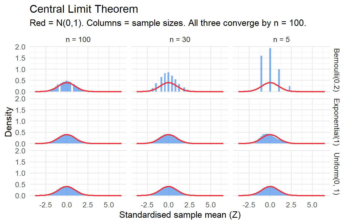
#| label: fig-clt-demo
#| fig-cap: "CLT: sampling distributions from three non-normal parents approach N(0,1) as n grows."
n_sims <- 10000

simulate_clt <- function(dist_fn, n_vals = c(5, 30, 100)) {
  map_dfr(n_vals, function(n) {
    tibble(n = n, x_bar = replicate(n_sims, mean(dist_fn(n))))
  })
}

bind_rows(
  simulate_clt(\(n) rexp(n, rate = 1))      |> mutate(dist = "Exponential(1)"),
  simulate_clt(\(n) rbinom(n, 1, 0.2))      |> mutate(dist = "Bernoulli(0.2)"),
  simulate_clt(\(n) runif(n, 0, 1))         |> mutate(dist = "Uniform(0, 1)")
) |>
  group_by(dist, n) |>
  mutate(z = (x_bar - mean(x_bar)) / sd(x_bar)) |>
  ggplot(aes(z)) +
  geom_histogram(aes(y = after_stat(density)), bins = 50,
                 fill = "#2c7be5", alpha = 0.6) +
  stat_function(fun = dnorm, colour = "#e63946", linewidth = 1) +
  facet_grid(dist ~ paste("n =", n)) +
  labs(x = "Standardised sample mean (Z)", y = "Density",
       title = "Central Limit Theorem",
       subtitle = "Red = N(0,1). Columns = sample sizes. All three converge by n = 100.")
```
---
## Consistency of OLS
### Scalar Case
Recall from Chapter 4: $\hat{\beta}_1 = \beta_1 + \frac{\frac{1}{n}\sum(x_i - \bar{x})u_i}{\frac{1}{n}\sum(x_i - \bar{x})^2}$.
By the WLLN (assuming i.i.d. observations):
$$\frac{1}{n}\sum(x_i - \bar{x})^2 \xrightarrow{p} \text{Var}(x) \equiv \sigma_x^2 > 0$$
$$\frac{1}{n}\sum(x_i - \bar{x})u_i \xrightarrow{p} \text{Cov}(x, u)$$
By the CMT (division is continuous away from zero):
$$\text{plim}(\hat{\beta}_1) = \beta_1 + \frac{\text{Cov}(x, u)}{\text{Var}(x)}$$
OLS is **consistent** if and only if $\text{Cov}(x, u) = 0$.
### Matrix Case
Write $\hat{\boldsymbol{\beta}} = \boldsymbol{\beta} + \left(\frac{\mathbf{X}'\mathbf{X}}{n}\right)^{-1}\left(\frac{\mathbf{X}'\mathbf{u}}{n}\right)$.
Define $\mathbf{Q}_{XX} = E[\mathbf{x}_i\mathbf{x}_i']$ (the population second-moment matrix of the regressors). By the WLLN applied to each element:
$$\frac{\mathbf{X}'\mathbf{X}}{n} = \frac{1}{n}\sum_{i=1}^n \mathbf{x}_i\mathbf{x}_i' \xrightarrow{p} \mathbf{Q}_{XX}$$
By MLR.4 ($E[\mathbf{u} \mid \mathbf{X}] = \mathbf{0}$, implying $E[\mathbf{x}_i u_i] = \mathbf{0}$):
$$\frac{\mathbf{X}'\mathbf{u}}{n} = \frac{1}{n}\sum_{i=1}^n \mathbf{x}_i u_i \xrightarrow{p} E[\mathbf{x}_i u_i] = \mathbf{0}$$
By the CMT (matrix inversion is continuous at invertible matrices, and $\mathbf{Q}_{XX}$ is invertible by MLR.3):
$$\text{plim}(\hat{\boldsymbol{\beta}}) = \boldsymbol{\beta} + \mathbf{Q}_{XX}^{-1} \cdot \mathbf{0} = \boldsymbol{\beta} \qquad \blacksquare$$
::: {.callout-important}
## Consistency vs. Unbiasedness
- **Unbiasedness**: $E[\hat{\boldsymbol{\beta}}] = \boldsymbol{\beta}$ for any fixed $n$ — requires $E[\mathbf{u} \mid \mathbf{X}] = \mathbf{0}$ (MLR.4)
- **Consistency**: $\hat{\boldsymbol{\beta}} \xrightarrow{p} \boldsymbol{\beta}$ — requires only $E[\mathbf{x}_i u_i] = \mathbf{0}$ (zero correlation, not zero conditional mean)
Zero conditional mean implies zero correlation (by LIE), but not vice versa. So consistency holds under strictly weaker conditions than unbiasedness. An estimator can be biased in finite samples but consistent (many instrumental variables estimators are in this category).
:::
---
## Asymptotic Normality of OLS
### Derivation
The key is to express $\sqrt{n}(\hat{\boldsymbol{\beta}} - \boldsymbol{\beta})$ as a function of a sample average and apply the CLT.
$$\sqrt{n}(\hat{\boldsymbol{\beta}} - \boldsymbol{\beta}) = \left(\frac{\mathbf{X}'\mathbf{X}}{n}\right)^{-1} \cdot \left(\frac{\mathbf{X}'\mathbf{u}}{\sqrt{n}}\right) = \left(\frac{\mathbf{X}'\mathbf{X}}{n}\right)^{-1} \cdot \left(\frac{1}{\sqrt{n}}\sum_{i=1}^n \mathbf{x}_i u_i\right)$$
**Step 1: Apply the CLT to the last factor.** Under MLR.1–5, $\{\mathbf{x}_i u_i\}$ are i.i.d. with mean $\mathbf{0}$ and covariance matrix:
$$E[\mathbf{x}_i u_i \mathbf{x}_i' u_i] = E[\mathbf{x}_i \mathbf{x}_i' u_i^2] = \sigma^2 E[\mathbf{x}_i \mathbf{x}_i'] = \sigma^2 \mathbf{Q}_{XX}$$
(using MLR.5: $E[u_i^2 \mid \mathbf{x}_i] = \sigma^2$). By the multivariate CLT:
$$\frac{1}{\sqrt{n}}\sum_{i=1}^n \mathbf{x}_i u_i \xrightarrow{d} \mathcal{N}(\mathbf{0},\, \sigma^2 \mathbf{Q}_{XX})$$
**Step 2: Apply Slutsky's theorem.** Since $\mathbf{X}'\mathbf{X}/n \xrightarrow{p} \mathbf{Q}_{XX}$ (consistent, hence converges in probability to a constant):
$$\sqrt{n}(\hat{\boldsymbol{\beta}} - \boldsymbol{\beta}) = \underbrace{\left(\frac{\mathbf{X}'\mathbf{X}}{n}\right)^{-1}}_{\xrightarrow{p}\;\mathbf{Q}_{XX}^{-1}} \cdot \underbrace{\left(\frac{1}{\sqrt{n}}\sum_{i=1}^n \mathbf{x}_i u_i\right)}_{\xrightarrow{d}\;\mathcal{N}(\mathbf{0},\,\sigma^2\mathbf{Q}_{XX})} \xrightarrow{d} \mathcal{N}\!\left(\mathbf{0},\; \sigma^2 \mathbf{Q}_{XX}^{-1}\right)$$
**Step 3: Normalise.** Dividing by $\sqrt{n}$:
$$\hat{\boldsymbol{\beta}} \overset{a}{\sim} \mathcal{N}\!\left(\boldsymbol{\beta},\; \frac{\sigma^2}{n} \mathbf{Q}_{XX}^{-1}\right)$$
Since $\sigma^2 \mathbf{Q}_{XX}^{-1}/n \approx \sigma^2(\mathbf{X}'\mathbf{X})^{-1}$ for large $n$, we recover:
$$\boxed{\hat{\boldsymbol{\beta}} \overset{a}{\sim} \mathcal{N}\!\left(\boldsymbol{\beta},\; \sigma^2(\mathbf{X}'\mathbf{X})^{-1}\right)}$$
This is the same variance formula as the exact finite-sample result under normality (Chapter 4) — but now derived without the normality assumption, valid for all large $n$.
### Asymptotic t-Tests
For a single coefficient:
$$\frac{\hat{\beta}_j - \beta_j}{\text{se}(\hat{\beta}_j)} \overset{a}{\sim} \mathcal{N}(0,1) \approx t(n-k-1)$$
For large $n$, $t(n-k-1) \approx \mathcal{N}(0,1)$, so the $t$-critical values converge to $z$-critical values (e.g., $t_{0.025,\infty} = 1.96$). In practice we always use the $t(n-k-1)$ critical values, which are conservative (heavier tails) and approach $\mathcal{N}(0,1)$ as $n$ grows.
### What Breaks Without Homoskedasticity?
If MLR.5 fails, let $\omega_i^2 = E[u_i^2 \mid \mathbf{x}_i]$ (the conditional variance, allowed to vary). Then:
$$\text{Cov}\!\left(\frac{1}{\sqrt{n}}\sum_{i=1}^n \mathbf{x}_i u_i\right) \xrightarrow{p} E[\mathbf{x}_i \mathbf{x}_i' u_i^2] = E[\omega_i^2 \mathbf{x}_i \mathbf{x}_i'] \neq \sigma^2 \mathbf{Q}_{XX}$$
The asymptotic distribution of $\hat{\boldsymbol{\beta}}$ becomes:
$$\sqrt{n}(\hat{\boldsymbol{\beta}} - \boldsymbol{\beta}) \xrightarrow{d} \mathcal{N}\!\left(\mathbf{0},\; \mathbf{Q}_{XX}^{-1} \boldsymbol{\Omega}\, \mathbf{Q}_{XX}^{-1}\right)$$
where $\boldsymbol{\Omega} = E[\omega_i^2 \mathbf{x}_i \mathbf{x}_i']$ is the "meat" of the sandwich. The homoskedastic formula $\sigma^2 \mathbf{Q}_{XX}^{-1}$ is now wrong. We need the **heteroskedasticity-robust (sandwich) estimator** of the variance — the topic of Chapter 9.
---
## Demonstrating Consistency via Simulation
```{r}
#| label: fig-consistency
#| fig-cap: "OLS consistency with non-normal errors: distribution concentrates on true value as n grows."
true_beta <- 0.5

results_n <- map_dfr(c(25, 100, 500, 2000, 10000), function(n) {
  slopes <- replicate(1000, {
    x <- runif(n, 0, 10)
    u <- rexp(n, rate = 1) - 1   # non-normal, mean zero
    y <- 1 + true_beta * x + u
    coef(lm(y ~ x))[2]
  })
  tibble(n = n, slope = slopes)
})

results_n |>
  group_by(n) |>
  summarise(mean = mean(slope), sd = sd(slope)) |>
  knitr::kable(digits = 4,
               caption = "OLS slope: mean and SD by sample size. Non-normal (Exponential) errors.")
```
```{r}
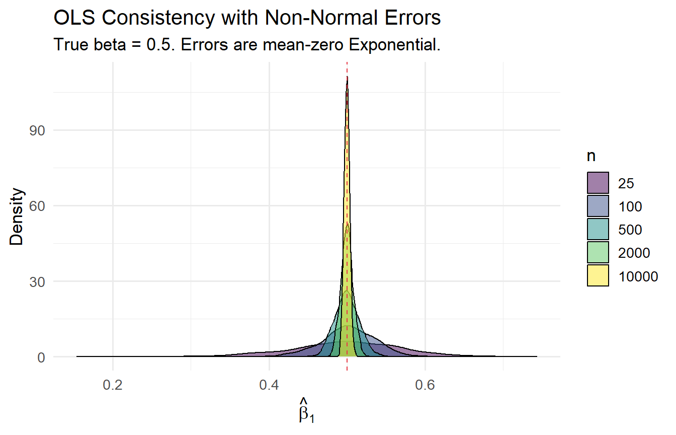
#| label: fig-consistency-plot
#| fig-cap: "The sampling distribution of β̂₁ narrows around the true value as n grows."
results_n |>
  ggplot(aes(slope, fill = factor(n))) +
  geom_density(alpha = 0.5) +
  geom_vline(xintercept = true_beta, linetype = "dashed", colour = "#e63946") +
  scale_fill_viridis_d(name = "n") +
  labs(x = expression(hat(beta)[1]), y = "Density",
       title = "OLS Consistency with Non-Normal Errors",
       subtitle = "True beta = 0.5. Errors are mean-zero Exponential.")
```
The distribution becomes increasingly concentrated around 0.5 as $n$ grows, confirming consistency with non-normal errors.
---
## Tutorials
**Tutorial 8.1**
Show via simulation that OLS is **inconsistent** when $\text{Cov}(x, u) \neq 0$. Let $u_i = 0.7 x_i + v_i$ where $v_i$ is independent noise. Before simulating, compute the theoretical probability limit.
::: {.callout-tip collapse="true"}
## Solution
```{r}
#| label: ex8-1
# plim(b1) = beta_1 + Cov(x,u)/Var(x)
# Cov(x, 0.7x + v) = 0.7*Var(x); Var(x) = 1 for N(0,1)
# plim = 0.5 + 0.7 = 1.2
cat("Theoretical plim(beta_hat):", 0.5 + 0.7, "\n\n")
for (n in c(100, 1000, 10000)) {
  slopes <- replicate(2000, {
    x <- rnorm(n); v <- rnorm(n)
    u <- 0.7 * x + v
    y <- 1 + 0.5 * x + u
    coef(lm(y ~ x))[2]
  })
  cat(sprintf("n = %6d:  mean slope = %.4f\n", n, mean(slopes)))
}
```
Even at $n = 10{,}000$, the estimate converges to 1.2 — not 0.5. Inconsistency is not solved by more data.
:::
**Tutorial 8.2**
The OLS slope can be written as $\hat{\beta}_1 = \beta_1 + \overline{(x_i - \bar{x})u_i} / \overline{(x_i - \bar{x})^2}$ where the bars denote averages. Use the WLLN and CMT to prove consistency in the scalar case. State precisely which assumptions you invoke at each step.
::: {.callout-tip collapse="true"}
## Solution
**Step 1 (WLLN on denominator).** Under random sampling (MLR.2) and $\text{Var}(x) < \infty$ (MLR.3):
$$\frac{1}{n}\sum(x_i - \bar{x})^2 \xrightarrow{p} E[(x_i - \mu_x)^2] = \text{Var}(x) > 0$$
The inequality is MLR.3 (no perfect collinearity).
**Step 2 (WLLN on numerator).** Under random sampling and MLR.4 ($E[u_i x_i] = E[u_i]\mu_x = 0$ since MLR.4 implies $E[u_i] = 0$ and $\text{Cov}(x_i, u_i) = 0$):
$$\frac{1}{n}\sum(x_i - \bar{x})u_i \xrightarrow{p} \text{Cov}(x_i, u_i) = 0$$
**Step 3 (CMT).** Since division is a continuous function and $\text{Var}(x) \neq 0$:
$$\hat{\beta}_1 = \beta_1 + \frac{\text{numerator}}{\text{denominator}} \xrightarrow{p} \beta_1 + \frac{0}{\text{Var}(x)} = \beta_1 \qquad \blacksquare$$
:::
**Tutorial 8.3**
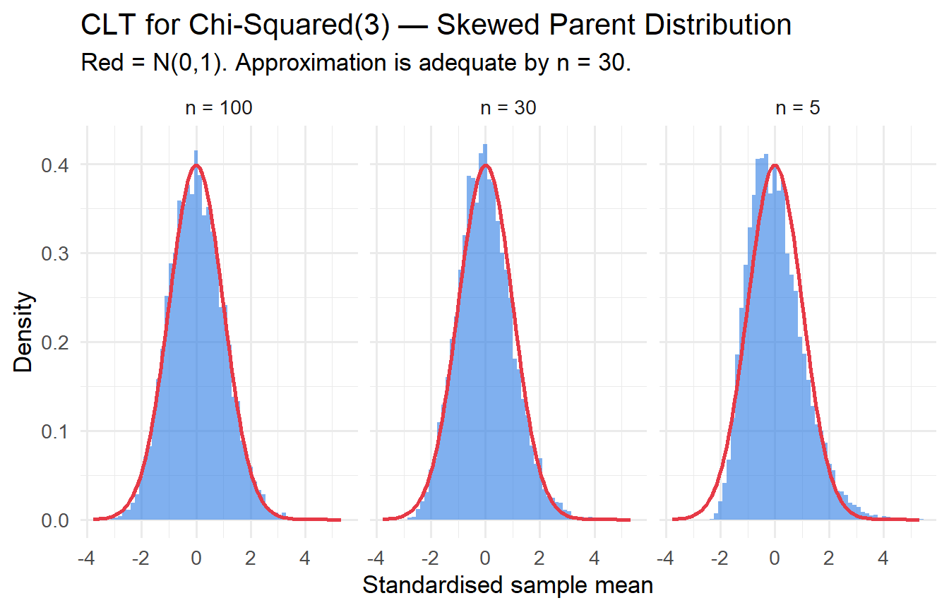
Simulate the CLT for the $\chi^2(3)$ distribution (highly non-normal, right-skewed). For $n \in \{5, 30, 100\}$, compute 10,000 sample means, standardise them, and overlay a $\mathcal{N}(0,1)$ density. At which $n$ does the approximation become adequate?
::: {.callout-tip collapse="true"}
## Solution
```{r}
#| label: ex8-3
#| fig-cap: "CLT for chi-squared(3) distribution: convergence to normality."
map_dfr(c(5, 30, 100), function(n) {
  x_bars <- replicate(10000, mean(rchisq(n, df = 3)))
  tibble(n = n, z = (x_bars - 3) / (sqrt(6/n)))   # mu=3, sigma^2=6
}) |>
  ggplot(aes(z)) +
  geom_histogram(aes(y = after_stat(density)), bins = 60,
                 fill = "#2c7be5", alpha = 0.6) +
  stat_function(fun = dnorm, colour = "#e63946", linewidth = 1) +
  facet_wrap(~paste("n =", n)) +
  labs(x = "Standardised sample mean", y = "Density",
       title = "CLT for Chi-Squared(3) — Skewed Parent Distribution",
       subtitle = "Red = N(0,1). Approximation is adequate by n = 30.")
```
For $\chi^2(3)$: $\mu = 3$, $\sigma^2 = 2\times 3 = 6$. The approximation is adequate by $n = 30$; at $n = 5$ the skewness of the parent distribution is still visible.
:::