Chapter 1: Introduction to Quantitative Methods

What, why, and how — with a first look at data in R

Learning Objectives

By the end of this chapter you will be able to:

Explain what quantitative methods do and why they matter for economics
Distinguish causality from correlation and describe why the distinction matters
Identify the main types of economic data
Load and explore a dataset in R using dplyr and ggplot2

1 What Are Quantitative Methods?

Economics is ultimately about understanding relationships: Does education raise wages? Does government spending stimulate growth? Do minimum wage laws reduce employment?

Answering these questions requires more than theory — we need data and methods to confront theory with evidence. Quantitative methods are the systematic procedures for doing so.

At the core of most empirical economics is regression analysis: a statistical technique that describes how one variable changes, on average, as another variable changes, holding other things constant.

The Central Goal

We want to estimate the causal effect of $X$ on $Y$ — the change in $Y$ that would result from an exogenous change in $X$, all else equal.

This is harder than it sounds.

2 Causality vs. Correlation

The most important distinction in empirical economics is between correlation and causation.

Two variables are correlated if they tend to move together. They are causally related if changing one produces a change in the other.

Example: Countries with more hospital beds per capita tend to have higher death rates. Does building more hospitals kill people?

No — sicker populations need more hospitals. The correlation is real; the causal interpretation is wrong. This is reverse causality.

2.1 The Gold Standard: Randomised Controlled Trials

The cleanest way to establish causality is a randomised controlled trial (RCT): randomly assign units to treatment and control, then compare outcomes.

Because randomisation balances all other factors (observed and unobserved) between groups, any difference in outcomes can be attributed to the treatment.

In economics, RCTs are often impossible (we cannot randomly assign countries to different tax regimes). Regression analysis is one tool for drawing causal conclusions from observational data — but it requires strong assumptions.

2.2 The Problem of Confounding

A confounder is a third variable that affects both $X$ and $Y$, creating a spurious correlation between them.

\[ Z \rightarrow X, \quad Z \rightarrow Y \implies X \text{ and } Y \text{ correlated (spuriously)} \]

Regression allows us to control for confounders — provided we can measure them. Unmeasured confounders remain a threat.

3 Types of Economic Data

Type	Description	Example
Cross-section	Many units, one point in time	Survey of 1,000 workers in 2023
Time series	One unit, many time periods	Australia’s GDP, 1960–2024
Pooled cross-section	Many units, multiple periods (not tracked)	Labour surveys 2018–2023
Panel (longitudinal)	Same units tracked over time	500 firms observed 2015–2023

Different data structures require different methods. This course focuses primarily on cross-sectional (Chapters 1–9) and time series (Chapters 10–12) data.

4 A First Look at Data in R

We will use the gapminder dataset — 142 countries observed every five years from 1952 to 2007, with GDP per capita, life expectancy, and population.

4.1 Loading and Inspecting

library(gapminder)

glimpse(gapminder)

Rows: 1,704
Columns: 6
$ country   <fct> "Afghanistan", "Afghanistan", "Afghanistan", "Afghanistan", …
$ continent <fct> Asia, Asia, Asia, Asia, Asia, Asia, Asia, Asia, Asia, Asia, …
$ year      <int> 1952, 1957, 1962, 1967, 1972, 1977, 1982, 1987, 1992, 1997, …
$ lifeExp   <dbl> 28.80, 30.33, 32.00, 34.02, 36.09, 38.44, 39.85, 40.82, 41.6…
$ pop       <int> 8425333, 9240934, 10267083, 11537966, 13079460, 14880372, 12…
$ gdpPercap <dbl> 779.4, 820.9, 853.1, 836.2, 740.0, 786.1, 978.0, 852.4, 649.…

gapminder |>
  filter(year == 2007) |>
  select(country, continent, lifeExp, gdpPercap) |>
  slice_head(n = 10)

4.2 Summarising by Group

gapminder |>
  filter(year == 2007) |>
  group_by(continent) |>
  summarise(
    countries    = n(),
    median_gdp   = median(gdpPercap),
    median_life  = median(lifeExp),
    .groups = "drop"
  ) |>
  arrange(desc(median_gdp))

4.3 Visualising: GDP and Life Expectancy

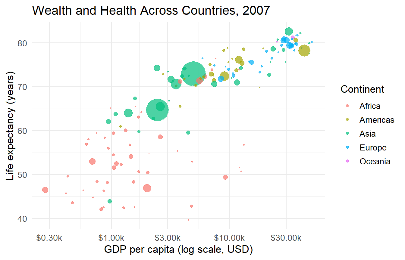
One of the most famous visualisations in economics is the relationship between income and health. Let’s reproduce it.

gapminder |>
  filter(year == 2007) |>
  ggplot(aes(x = gdpPercap, y = lifeExp,
             size = pop, colour = continent)) +
  geom_point(alpha = 0.7) +
  scale_x_log10(labels = scales::label_dollar(scale = 1e-3, suffix = "k")) +
  scale_size_area(max_size = 14, guide = "none") +
  labs(
    x      = "GDP per capita (log scale, USD)",
    y      = "Life expectancy (years)",
    colour = "Continent",
    title  = "Wealth and Health Across Countries, 2007"
  )

Figure 1: GDP per capita and life expectancy, 2007. Bubble size = population.

The positive relationship is clear, but note:

The log scale on the x-axis — the relationship is closer to linear in log GDP
Africa clusters at lower income and lower life expectancy
Some high-income countries (Gulf states) have lower life expectancy than you might expect given their wealth

4.4 A Simple Regression Line

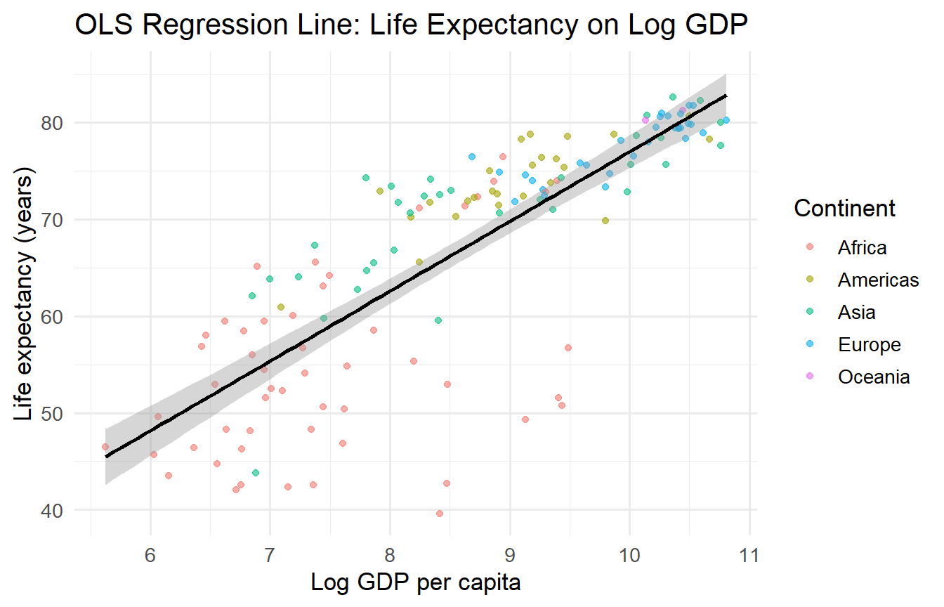
gapminder |>
  filter(year == 2007) |>
  mutate(log_gdp = log(gdpPercap)) |>
  ggplot(aes(x = log_gdp, y = lifeExp)) +
  geom_point(aes(colour = continent), alpha = 0.6) +
  geom_smooth(method = "lm", colour = "black", linewidth = 1) +
  labs(
    x      = "Log GDP per capita",
    y      = "Life expectancy (years)",
    colour = "Continent",
    title  = "OLS Regression Line: Life Expectancy on Log GDP"
  )

Figure 2: A linear regression of life expectancy on log GDP per capita.

The black line is an OLS regression line — the best-fitting straight line through these points. Over the next several chapters, we will learn exactly what “best-fitting” means, how to estimate it, and what we can infer from it.

5 The Regression Framework (Preview)

The regression model we will study is:

\[ y_i = \beta_0 + \beta_1 x_i + u_i \]

where:

$y_i$ is the dependent variable (outcome) for observation $i$
$x_i$ is the independent variable (regressor, predictor)
$\beta_0$ is the intercept — the expected value of $y$ when $x = 0$
$\beta_1$ is the slope — the change in $y$ for a one-unit increase in $x$
$u_i$ is the error term — everything that determines $y$ other than $x$

OLS finds the values $\hat{\beta}_0$ and $\hat{\beta}_1$ that minimise the sum of squared residuals $\sum_{i=1}^n \hat{u}_i^2$.

We will derive this properly in Chapter 3. For now, here is how to fit it in R:

data_2007 <- gapminder |>
  filter(year == 2007) |>
  mutate(log_gdp = log(gdpPercap))

fit <- lm(lifeExp ~ log_gdp, data = data_2007)
tidy(fit)

The slope of 7.2 means: a 1-unit increase in log GDP per capita is associated with approximately 7.2 additional years of life expectancy. We will learn how to interpret, test, and critique this estimate thoroughly.

6 The Conditional Expectation Function

Regression has a deeper interpretation than “best-fitting line.” The Conditional Expectation Function (CEF):

\[m(x) = E[y \mid x]\]

is the population average of $y$ given a particular value of $x$. The CEF is the true relationship that regression estimates.

Why the CEF? The CEF is the best predictor of $y$ given $x$ in the mean-squared error sense: $E[y \mid x]$ minimises $E[(y - g(x))^2]$ over all functions $g$. Any regression — linear or non-linear — attempts to approximate the CEF.

When the CEF is linear (i.e., $E[y \mid x] = \beta_0 + \beta_1 x$), OLS recovers the exact population relationship. When the CEF is non-linear, OLS provides the best linear approximation to it.

The error term. Define $u_i = y_i - E[y_i \mid x_i]$. By construction:

\[E[u_i \mid x_i] = E[y_i - E[y_i \mid x_i] \mid x_i] = E[y_i \mid x_i] - E[y_i \mid x_i] = 0\]

The zero conditional mean $E[u \mid x] = 0$ is not an assumption about the world — it is a definition of the error term as the deviation from the CEF. The substantive assumption is that $E[y \mid x]$ is what we claim it is (e.g., linear, with specific regressors included).

6.1 Prediction vs. Causal Inference

The CEF supports two different research goals:

Prediction: Given a new observation $x_0$, predict $y_0$. We want $\hat{y}_0 \approx E[y \mid x_0]$ with low error. Here, $\hat{\beta}$ does not need to represent a causal effect — it just needs to predict well.

Causal inference: What would happen to $y$ if we intervened to change $x$ by one unit? This is the average treatment effect (ATE) or average causal effect. For OLS to recover a causal effect, we need $E[u \mid x] = 0$ to hold not just as a definitional tautology, but because there are genuinely no omitted confounders correlated with $x$.

The Key Distinction

A good prediction model can use any correlated variable — it doesn’t matter if the correlation is causal. A good causal model must isolate the variation in $x$ that is exogenous (not caused by $y$ and not correlated with omitted variables). These two goals can require very different modelling choices.

7 Identification Problems

In observational data, the relationship between $x$ and $y$ is confounded by three types of problems:

1. Omitted Variable Bias (OVB). An unobserved third variable $z$ affects both $x$ and $y$: \[z \to x, \quad z \to y\] Example: Ability raises both education and wages. Regressing wages on education overstates the return to education by picking up the effect of ability.

2. Reverse Causality. $y$ causes $x$, not just $x$ causes $y$: \[y \to x\] Example: Firms with high sales may hire more workers. Regressing workers on sales confounds the effect of workers on output with the effect of output on hiring decisions.

3. Simultaneous Causality. $x$ causes $y$ and $y$ causes $x$ simultaneously — a system of equations. This is distinct from reverse causality: \[x \to y \text{ and } y \to x \text{ (simultaneously)}\] Example: Demand ($q$) and price ($p$) are simultaneously determined by supply and demand in equilibrium. Regressing $q$ on $p$ (or $p$ on $q$) gives neither a supply nor a demand elasticity — it gives a mixture that reflects the simultaneous system.

All three problems cause $\text{Cov}(x, u) \neq 0$, which means OLS estimates are biased and inconsistent. The identification strategies that address them — instrumental variables, regression discontinuity, difference-in-differences, randomised assignment — are the frontier of modern applied econometrics.

8 How Time Has Changed This Relationship

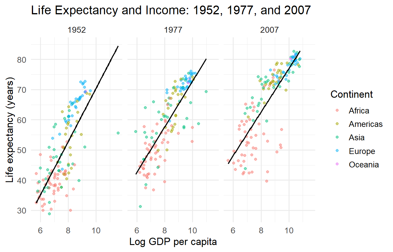
gapminder |>
  filter(year %in% c(1952, 1977, 2007)) |>
  mutate(log_gdp = log(gdpPercap)) |>
  ggplot(aes(x = log_gdp, y = lifeExp, colour = continent)) +
  geom_point(alpha = 0.5, size = 1.5) +
  geom_smooth(method = "lm", se = FALSE, colour = "black", linewidth = 0.8) +
  facet_wrap(~year) +
  labs(
    x      = "Log GDP per capita",
    y      = "Life expectancy (years)",
    colour = "Continent",
    title  = "Life Expectancy and Income: 1952, 1977, and 2007"
  )

Figure 3: The income-health relationship shifting over time.

Life expectancy has risen substantially at all income levels — this is the level shift. The slope of the relationship (the return to income in terms of health) has changed too. Panel data methods (beyond this course) allow us to study both.

9 Tutorials

Tutorial 1.1 Using the gapminder data, calculate the average life expectancy and GDP per capita for each continent in 1952 and 2007. By how much has each improved? Which continent saw the largest absolute improvement in life expectancy?

Solution

gapminder |>
  filter(year %in% c(1952, 2007)) |>
  group_by(continent, year) |>
  summarise(
    mean_life = mean(lifeExp),
    mean_gdp  = mean(gdpPercap),
    .groups = "drop"
  ) |>
  pivot_wider(
    names_from  = year,
    values_from = c(mean_life, mean_gdp)
  ) |>
  mutate(life_improvement = mean_life_2007 - mean_life_1952) |>
  arrange(desc(life_improvement))

Africa saw the largest absolute improvement in life expectancy (approximately 15 years), though it still lags other continents considerably.

Tutorial 1.2 Identify a research question in economics (from your field of interest or a published paper). For each:

What is the dependent variable $Y$?
What is the key independent variable $X$?
What are plausible confounders that might make the OLS estimate of the effect of $X$ on $Y$ misleading?
Is an RCT feasible? If not, what alternative identification strategies might work?

Example Answer

Question: Does attending university increase earnings?

$Y$: Annual earnings 10 years after completing school
$X$: University attendance (yes/no)
Confounders: Ability (smarter people both go to university and earn more), family background, field of study choice, access to networks
RCT feasibility: Randomly denying access to university is unethical and impractical
Alternative strategies: Instrumental variables (e.g., distance to nearest university as an instrument for attendance), regression discontinuity (exploiting cut-off scores for admission), twin studies

Tutorial 1.3 For each scenario, state whether the most plausible concern is reverse causality, omitted variable bias, or measurement error:

A study finds that firms with more HR staff have lower productivity.
A regression of health on income uses self-reported income.
Cities with more police have higher crime rates.

Solution

Reverse causality: Low-productivity firms may hire more HR staff to manage poor performance, not vice versa.
Measurement error: Self-reported income is often inaccurately recalled; measurement error in $X$ biases the OLS estimate towards zero (attenuation bias).
Reverse causality (or omitted variable bias): High-crime cities attract more policing investment; the causal effect of police may still be negative, but the OLS estimate confounds it with the reverse flow.

10 Key Terms

Term	Definition
Regression analysis	Statistical technique for estimating the relationship between a dependent variable and one or more independent variables
OLS	Ordinary Least Squares — the estimator that minimises the sum of squared residuals
Causality	$X$ causes $Y$ if an exogenous change in $X$ produces a change in $Y$
Confounder	A variable that affects both $X$ and $Y$, creating spurious correlation
Cross-section data	Data on multiple units observed at a single point in time
Time series data	Data on a single unit observed across multiple time periods

--- title: "Chapter 1: Introduction to Quantitative Methods" subtitle: "What, why, and how — with a first look at data in R" --- ```{r} #| label: setup #| include: false library(tidyverse) library(gapminder) library(broom) library(modelsummary) theme_set(theme_minimal(base_size = 13)) options(digits = 4, scipen = 999) ``` ::: {.callout-note} ## Learning Objectives By the end of this chapter you will be able to: - Explain what quantitative methods do and why they matter for economics - Distinguish causality from correlation and describe why the distinction matters - Identify the main types of economic data - Load and explore a dataset in R using `dplyr` and `ggplot2` ::: --- ## What Are Quantitative Methods? Economics is ultimately about understanding relationships: Does education raise wages? Does government spending stimulate growth? Do minimum wage laws reduce employment? Answering these questions requires more than theory — we need data and methods to confront theory with evidence. **Quantitative methods** are the systematic procedures for doing so. At the core of most empirical economics is **regression analysis**: a statistical technique that describes how one variable changes, on average, as another variable changes, holding other things constant. ::: {.callout-tip} ## The Central Goal We want to estimate the **causal effect** of $X$ on $Y$ — the change in $Y$ that *would result* from an exogenous change in $X$, all else equal. This is harder than it sounds. ::: --- ## Causality vs. Correlation The most important distinction in empirical economics is between **correlation** and **causation**. Two variables are *correlated* if they tend to move together. They are *causally related* if changing one *produces* a change in the other. **Example:** Countries with more hospital beds per capita tend to have higher death rates. Does building more hospitals kill people? No — sicker populations need more hospitals. The correlation is real; the causal interpretation is wrong. This is **reverse causality**. ### The Gold Standard: Randomised Controlled Trials The cleanest way to establish causality is a **randomised controlled trial (RCT)**: randomly assign units to treatment and control, then compare outcomes. Because randomisation balances all other factors (observed and unobserved) between groups, any difference in outcomes can be attributed to the treatment. In economics, RCTs are often impossible (we cannot randomly assign countries to different tax regimes). Regression analysis is one tool for drawing causal conclusions from observational data — but it requires strong assumptions. ### The Problem of Confounding A **confounder** is a third variable that affects both $X$ and $Y$, creating a spurious correlation between them. $$ Z \rightarrow X, \quad Z \rightarrow Y \implies X \text{ and } Y \text{ correlated (spuriously)} $$ Regression allows us to **control for** confounders — provided we can measure them. Unmeasured confounders remain a threat. --- ## Types of Economic Data | Type | Description | Example | |------|-------------|---------| | **Cross-section** | Many units, one point in time | Survey of 1,000 workers in 2023 | | **Time series** | One unit, many time periods | Australia's GDP, 1960–2024 | | **Pooled cross-section** | Many units, multiple periods (not tracked) | Labour surveys 2018–2023 | | **Panel (longitudinal)** | Same units tracked over time | 500 firms observed 2015–2023 | Different data structures require different methods. This course focuses primarily on **cross-sectional** (Chapters 1–9) and **time series** (Chapters 10–12) data. --- ## A First Look at Data in R We will use the `gapminder` dataset — 142 countries observed every five years from 1952 to 2007, with GDP per capita, life expectancy, and population. ### Loading and Inspecting ```{r} #| label: gapminder-glimpse library(gapminder) glimpse(gapminder) ``` ```{r} #| label: gapminder-summary gapminder |> filter(year == 2007) |> select(country, continent, lifeExp, gdpPercap) |> slice_head(n = 10) ``` ### Summarising by Group ```{r} #| label: gapminder-grouped gapminder |> filter(year == 2007) |> group_by(continent) |> summarise( countries = n(), median_gdp = median(gdpPercap), median_life = median(lifeExp), .groups = "drop" ) |> arrange(desc(median_gdp)) ``` ### Visualising: GDP and Life Expectancy One of the most famous visualisations in economics is the relationship between income and health. Let's reproduce it. ```{r} #| label: fig-gapminder-scatter #| fig-cap: "GDP per capita and life expectancy, 2007. Bubble size = population." gapminder |> filter(year == 2007) |> ggplot(aes(x = gdpPercap, y = lifeExp, size = pop, colour = continent)) + geom_point(alpha = 0.7) + scale_x_log10(labels = scales::label_dollar(scale = 1e-3, suffix = "k")) + scale_size_area(max_size = 14, guide = "none") + labs( x = "GDP per capita (log scale, USD)", y = "Life expectancy (years)", colour = "Continent", title = "Wealth and Health Across Countries, 2007" ) ``` The positive relationship is clear, but note: 1. The **log scale** on the x-axis — the relationship is closer to linear in log GDP 2. **Africa** clusters at lower income and lower life expectancy 3. Some high-income countries (Gulf states) have lower life expectancy than you might expect given their wealth ### A Simple Regression Line ```{r} #| label: fig-gapminder-lm #| fig-cap: "A linear regression of life expectancy on log GDP per capita." gapminder |> filter(year == 2007) |> mutate(log_gdp = log(gdpPercap)) |> ggplot(aes(x = log_gdp, y = lifeExp)) + geom_point(aes(colour = continent), alpha = 0.6) + geom_smooth(method = "lm", colour = "black", linewidth = 1) + labs( x = "Log GDP per capita", y = "Life expectancy (years)", colour = "Continent", title = "OLS Regression Line: Life Expectancy on Log GDP" ) ``` The black line is an **OLS regression line** — the best-fitting straight line through these points. Over the next several chapters, we will learn exactly what "best-fitting" means, how to estimate it, and what we can infer from it. --- ## The Regression Framework (Preview) The regression model we will study is: $$ y_i = \beta_0 + \beta_1 x_i + u_i $$ where: - $y_i$ is the **dependent variable** (outcome) for observation $i$ - $x_i$ is the **independent variable** (regressor, predictor) - $\beta_0$ is the **intercept** — the expected value of $y$ when $x = 0$ - $\beta_1$ is the **slope** — the change in $y$ for a one-unit increase in $x$ - $u_i$ is the **error term** — everything that determines $y$ other than $x$ OLS finds the values $\hat{\beta}_0$ and $\hat{\beta}_1$ that minimise the sum of squared residuals $\sum_{i=1}^n \hat{u}_i^2$. We will derive this properly in Chapter 3. For now, here is how to fit it in R: ```{r} #| label: first-regression data_2007 <- gapminder |> filter(year == 2007) |> mutate(log_gdp = log(gdpPercap)) fit <- lm(lifeExp ~ log_gdp, data = data_2007) tidy(fit) ``` The slope of **`r round(coef(fit)[2], 2)`** means: a 1-unit increase in log GDP per capita is associated with approximately `r round(coef(fit)[2], 2)` additional years of life expectancy. We will learn how to interpret, test, and critique this estimate thoroughly. --- ## The Conditional Expectation Function Regression has a deeper interpretation than "best-fitting line." The **Conditional Expectation Function (CEF)**: $$m(x) = E[y \mid x]$$ is the population average of $y$ given a particular value of $x$. The CEF is the true relationship that regression estimates. **Why the CEF?** The CEF is the best predictor of $y$ given $x$ in the mean-squared error sense: $E[y \mid x]$ minimises $E[(y - g(x))^2]$ over all functions $g$. Any regression — linear or non-linear — attempts to approximate the CEF. When the CEF is linear (i.e., $E[y \mid x] = \beta_0 + \beta_1 x$), OLS recovers the exact population relationship. When the CEF is non-linear, OLS provides the **best linear approximation** to it. **The error term.** Define $u_i = y_i - E[y_i \mid x_i]$. By construction: $$E[u_i \mid x_i] = E[y_i - E[y_i \mid x_i] \mid x_i] = E[y_i \mid x_i] - E[y_i \mid x_i] = 0$$ The zero conditional mean $E[u \mid x] = 0$ is not an assumption about the world — it is a **definition** of the error term as the deviation from the CEF. The substantive assumption is that $E[y \mid x]$ is what we claim it is (e.g., linear, with specific regressors included). ### Prediction vs. Causal Inference The CEF supports two different research goals: **Prediction:** Given a new observation $x_0$, predict $y_0$. We want $\hat{y}_0 \approx E[y \mid x_0]$ with low error. Here, $\hat{\beta}$ does not need to represent a causal effect — it just needs to predict well. **Causal inference:** What would happen to $y$ if we *intervened* to change $x$ by one unit? This is the **average treatment effect** (ATE) or **average causal effect**. For OLS to recover a causal effect, we need $E[u \mid x] = 0$ to hold not just as a definitional tautology, but because there are genuinely no omitted confounders correlated with $x$. ::: {.callout-important} ## The Key Distinction A good prediction model can use any correlated variable — it doesn't matter if the correlation is causal. A good causal model must isolate the variation in $x$ that is exogenous (not caused by $y$ and not correlated with omitted variables). These two goals can require very different modelling choices. ::: --- ## Identification Problems In observational data, the relationship between $x$ and $y$ is confounded by three types of problems: **1. Omitted Variable Bias (OVB).** An unobserved third variable $z$ affects both $x$ and $y$: $$z \to x, \quad z \to y$$ Example: Ability raises both education and wages. Regressing wages on education overstates the return to education by picking up the effect of ability. **2. Reverse Causality.** $y$ causes $x$, not just $x$ causes $y$: $$y \to x$$ Example: Firms with high sales may hire more workers. Regressing workers on sales confounds the effect of workers on output with the effect of output on hiring decisions. **3. Simultaneous Causality.** $x$ causes $y$ **and** $y$ causes $x$ simultaneously — a system of equations. This is distinct from reverse causality: $$x \to y \text{ and } y \to x \text{ (simultaneously)}$$ Example: Demand ($q$) and price ($p$) are simultaneously determined by supply and demand in equilibrium. Regressing $q$ on $p$ (or $p$ on $q$) gives neither a supply nor a demand elasticity — it gives a mixture that reflects the simultaneous system. All three problems cause $\text{Cov}(x, u) \neq 0$, which means OLS estimates are biased and inconsistent. The identification strategies that address them — instrumental variables, regression discontinuity, difference-in-differences, randomised assignment — are the frontier of modern applied econometrics. --- ## How Time Has Changed This Relationship ```{r} #| label: fig-gapminder-time #| fig-cap: "The income-health relationship shifting over time." gapminder |> filter(year %in% c(1952, 1977, 2007)) |> mutate(log_gdp = log(gdpPercap)) |> ggplot(aes(x = log_gdp, y = lifeExp, colour = continent)) + geom_point(alpha = 0.5, size = 1.5) + geom_smooth(method = "lm", se = FALSE, colour = "black", linewidth = 0.8) + facet_wrap(~year) + labs( x = "Log GDP per capita", y = "Life expectancy (years)", colour = "Continent", title = "Life Expectancy and Income: 1952, 1977, and 2007" ) ``` Life expectancy has risen substantially at all income levels — this is the **level shift**. The slope of the relationship (the return to income in terms of health) has changed too. Panel data methods (beyond this course) allow us to study both. --- ## Tutorials **Tutorial 1.1** Using the `gapminder` data, calculate the average life expectancy and GDP per capita for each continent in 1952 and 2007. By how much has each improved? Which continent saw the largest absolute improvement in life expectancy? ::: {.callout-tip collapse="true"} ## Solution ```{r} #| label: ex1-solution gapminder |> filter(year %in% c(1952, 2007)) |> group_by(continent, year) |> summarise( mean_life = mean(lifeExp), mean_gdp = mean(gdpPercap), .groups = "drop" ) |> pivot_wider( names_from = year, values_from = c(mean_life, mean_gdp) ) |> mutate(life_improvement = mean_life_2007 - mean_life_1952) |> arrange(desc(life_improvement)) ``` Africa saw the largest absolute improvement in life expectancy (approximately 15 years), though it still lags other continents considerably. ::: **Tutorial 1.2** Identify a research question in economics (from your field of interest or a published paper). For each: a. What is the dependent variable $Y$? b. What is the key independent variable $X$? c. What are plausible confounders that might make the OLS estimate of the effect of $X$ on $Y$ misleading? d. Is an RCT feasible? If not, what alternative identification strategies might work? ::: {.callout-tip collapse="true"} ## Example Answer **Question:** Does attending university increase earnings? - $Y$: Annual earnings 10 years after completing school - $X$: University attendance (yes/no) - **Confounders:** Ability (smarter people both go to university *and* earn more), family background, field of study choice, access to networks - **RCT feasibility:** Randomly denying access to university is unethical and impractical - **Alternative strategies:** Instrumental variables (e.g., distance to nearest university as an instrument for attendance), regression discontinuity (exploiting cut-off scores for admission), twin studies ::: **Tutorial 1.3** For each scenario, state whether the most plausible concern is **reverse causality**, **omitted variable bias**, or **measurement error**: a. A study finds that firms with more HR staff have lower productivity. b. A regression of health on income uses self-reported income. c. Cities with more police have higher crime rates. ::: {.callout-tip collapse="true"} ## Solution a. **Reverse causality**: Low-productivity firms may hire more HR staff to manage poor performance, not vice versa. b. **Measurement error**: Self-reported income is often inaccurately recalled; measurement error in $X$ biases the OLS estimate towards zero (attenuation bias). c. **Reverse causality** (or omitted variable bias): High-crime cities attract more policing investment; the causal effect of police may still be negative, but the OLS estimate confounds it with the reverse flow. ::: --- ## Key Terms | Term | Definition | |------|-----------| | **Regression analysis** | Statistical technique for estimating the relationship between a dependent variable and one or more independent variables | | **OLS** | Ordinary Least Squares — the estimator that minimises the sum of squared residuals | | **Causality** | $X$ causes $Y$ if an exogenous change in $X$ produces a change in $Y$ | | **Confounder** | A variable that affects both $X$ and $Y$, creating spurious correlation | | **Cross-section data** | Data on multiple units observed at a single point in time | | **Time series data** | Data on a single unit observed across multiple time periods |