fit <- lm(wage ~ educ + exper + tenure, data = wage1)
tidy(fit, conf.int = TRUE)Chapter 5: Inference and Hypothesis Testing
t-tests, F-tests, confidence intervals, and joint hypotheses
NoteLearning Objectives
By the end of this chapter you will be able to:
- Explain why OLS estimators have a normal sampling distribution under CLM.1–6
- Derive why we use the \(t\)-distribution rather than the standard normal
- Follow and apply the formal six-step hypothesis testing protocol
- Construct and interpret \(t\)-tests and confidence intervals for regression parameters
- Derive the \(F\)-statistic in both the SSR-ratio form and the \(R^2\) form
- Conduct \(F\)-tests for joint hypotheses using
car::linearHypothesis() - Use the reparameterisation trick to test non-zero null hypotheses and linear combinations
1 Normality of OLS Estimators
1.1 Why \(\hat{\boldsymbol{\beta}}\) is Normally Distributed
Under the full Classical Linear Model (CLM.1–6), we assume:
\[\mathbf{u} \mid \mathbf{X} \sim \mathcal{N}(\mathbf{0},\, \sigma^2 \mathbf{I}_n)\]
From Chapter 4 we showed that:
\[\hat{\boldsymbol{\beta}} = \boldsymbol{\beta} + (\mathbf{X}'\mathbf{X})^{-1}\mathbf{X}'\mathbf{u}\]
This is a linear transformation of the random vector \(\mathbf{u}\). A fundamental result from probability theory states that any affine transformation of a multivariate normal random vector is itself multivariate normal. Specifically, if \(\mathbf{u} \sim \mathcal{N}(\boldsymbol{\mu}, \boldsymbol{\Sigma})\) and \(\mathbf{A}\) is a fixed matrix, then \(\mathbf{A}\mathbf{u} \sim \mathcal{N}(\mathbf{A}\boldsymbol{\mu}, \mathbf{A}\boldsymbol{\Sigma}\mathbf{A}')\).
Applying this with \(\mathbf{A} = (\mathbf{X}'\mathbf{X})^{-1}\mathbf{X}'\):
\[\hat{\boldsymbol{\beta}} \mid \mathbf{X} \sim \mathcal{N}\!\left(\boldsymbol{\beta},\; \sigma^2 (\mathbf{X}'\mathbf{X})^{-1}\right)\]
This is an exact finite-sample result — it holds for any \(n\), not just asymptotically. In particular, each individual coefficient:
\[\hat{\beta}_j \mid \mathbf{X} \sim \mathcal{N}\!\left(\beta_j,\; \sigma^2 [(\mathbf{X}'\mathbf{X})^{-1}]_{jj}\right)\]
Standardising:
\[\frac{\hat{\beta}_j - \beta_j}{\sqrt{\sigma^2 [(\mathbf{X}'\mathbf{X})^{-1}]_{jj}}} \sim \mathcal{N}(0,1) \quad \text{exactly}\]
1.2 Why \(t\), Not \(Z\)
The standard normal pivot above is infeasible because \(\sigma^2\) is unknown. We replace it with \(\hat{\sigma}^2 = SSR/(n-k-1)\).
The key result is that under CLM.1–6:
\[\frac{SSR}{\sigma^2} = \frac{\hat{\mathbf{u}}'\hat{\mathbf{u}}}{\sigma^2} \sim \chi^2(n-k-1)\]
This follows because \(\hat{\mathbf{u}} = \mathbf{M}_X \mathbf{u}\), where \(\mathbf{M}_X\) is idempotent with rank \(n-k-1\), and a quadratic form in a normal vector with an idempotent matrix of rank \(r\) is \(\chi^2(r)\).
Moreover, \(\hat{\boldsymbol{\beta}}\) and \(\hat{\sigma}^2\) are independent (a result specific to the normal model: \(\hat{\boldsymbol{\beta}} = \boldsymbol{\beta} + \mathbf{P}_X \mathbf{u}\) and \(\hat{\mathbf{u}} = \mathbf{M}_X \mathbf{u}\) are orthogonal projections, and under normality orthogonality implies independence).
By definition, the ratio of a standard normal to the square root of an independent \(\chi^2(m)/m\) is a \(t(m)\) random variable:
\[t_j = \frac{(\hat{\beta}_j - \beta_j)/\sqrt{\sigma^2 [(\mathbf{X}'\mathbf{X})^{-1}]_{jj}}}{\sqrt{\hat{\sigma}^2/\sigma^2}} = \frac{\hat{\beta}_j - \beta_j}{\text{se}(\hat{\beta}_j)} \sim t(n-k-1)\]
where \(\text{se}(\hat{\beta}_j) = \hat{\sigma}\sqrt{[(\mathbf{X}'\mathbf{X})^{-1}]_{jj}}\).
The \(t\)-distribution has heavier tails than the standard normal, reflecting the additional uncertainty from estimating \(\sigma^2\). As \(n \to \infty\), \(\hat{\sigma}^2 \to \sigma^2\) and \(t(n-k-1) \to \mathcal{N}(0,1)\), so the distinction becomes irrelevant asymptotically.
2 Standard Errors
Under MLR.1–5, \(\text{Var}(\hat{\boldsymbol{\beta}} \mid \mathbf{X}) = \sigma^2(\mathbf{X}'\mathbf{X})^{-1}\). The standard error of \(\hat{\beta}_j\) is the square root of the \(j\)-th diagonal element of the estimated variance-covariance matrix:
\[\text{se}(\hat{\beta}_j) = \hat{\sigma}\sqrt{\left[(\mathbf{X}'\mathbf{X})^{-1}\right]_{jj}}\]
This is what lm() reports in the Std. Error column. It measures how much \(\hat{\beta}_j\) would vary across repeated samples of the same size from the same DGP.
3 The Six-Step Hypothesis Testing Protocol
Every hypothesis test in econometrics follows the same formal structure. Internalise it once and apply it everywhere.
Step 1: State the null and alternative hypotheses.
Be precise. A null hypothesis is a restriction on the population parameters, not on the estimates. Example: \(H_0: \beta_{educ} = 0\) vs. \(H_1: \beta_{educ} \neq 0\).
Step 2: Choose the test statistic and its null distribution.
For a single coefficient: \(t = (\hat{\beta}_j - \beta_j^0) / \text{se}(\hat{\beta}_j) \sim t(n-k-1)\) under \(H_0\).
Step 3: Set the significance level \(\alpha\).
The significance level is the maximum acceptable probability of a Type I error (rejecting \(H_0\) when it is true). Convention uses \(\alpha = 0.05\) or \(\alpha = 0.01\).
Step 4: Determine the rejection region (or equivalently, the critical value).
- Two-tailed \(H_1: \beta_j \neq \beta_j^0\): reject if \(|t| > t_{\alpha/2, n-k-1}\)
- One-tailed \(H_1: \beta_j > \beta_j^0\): reject if \(t > t_{\alpha, n-k-1}\)
- One-tailed \(H_1: \beta_j < \beta_j^0\): reject if \(t < -t_{\alpha, n-k-1}\)
Step 5: Compute the test statistic from the data.
Plug in the estimates. The test statistic is a number.
Step 6: State the conclusion.
Compare the test statistic to the critical value (or the p-value to \(\alpha\)). State whether you reject \(H_0\), at what significance level, and what this implies substantively.
Importantp-Values
The p-value is the probability of observing a test statistic at least as extreme as the one computed, assuming \(H_0\) is true. A small p-value is evidence against \(H_0\), not evidence for the alternative. Rejecting at the 5% level means: if \(H_0\) were true, we would see this result or something more extreme in fewer than 5% of samples.
4 Testing Individual Coefficients
Each row reports \(\hat{\beta}_j\), \(\text{se}(\hat{\beta}_j)\), \(t = \hat{\beta}_j / \text{se}(\hat{\beta}_j)\), the two-tailed p-value, and the 95% confidence interval. Applying the six-step protocol to educ:
- \(H_0: \beta_{educ} = 0\) vs. \(H_1: \beta_{educ} \neq 0\)
- \(t = \hat{\beta}_{educ} / \text{se}(\hat{\beta}_{educ}) \sim t(n-4)\) under \(H_0\)
- \(\alpha = 0.05\)
- Reject if \(|t| > t_{0.025, n-4}\)
- From the output: \(t \approx\) 11.68
- Since \(|t| \gg t_{0.025}\), we strongly reject \(H_0\). Education is significantly associated with wages, controlling for experience and tenure.
n <- nrow(wage1)
k <- 3
cat("Critical value (5%, two-tailed):", round(qt(0.975, df = n - k - 1), 3), "\n")
Critical value (5%, two-tailed): 1.965 5 Confidence Intervals
A \((1-\alpha) \times 100\%\) confidence interval for \(\beta_j\) is:
\[\hat{\beta}_j \pm t_{\alpha/2,\, n-k-1} \cdot \text{se}(\hat{\beta}_j)\]
The correct interpretation: if we were to repeat the sampling and estimation procedure many times, \((1-\alpha) \times 100\%\) of the resulting intervals would contain the true \(\beta_j\). This is a property of the procedure, not of any single interval.
confint(fit, level = 0.95) 2.5 % 97.5 %
(Intercept) -4.304799 -1.44067
educ 0.498218 0.69971
exper -0.001346 0.04603
tenure 0.126747 0.21179tidy(fit, conf.int = TRUE) |>
dplyr::filter(term != "(Intercept)") |>
ggplot(aes(y = term, x = estimate, xmin = conf.low, xmax = conf.high)) +
geom_errorbarh(height = 0.2, colour = "#2c7be5", linewidth = 1) +
geom_point(size = 3, colour = "#2c7be5") +
geom_vline(xintercept = 0, linetype = "dashed", colour = "#e63946") +
labs(x = "Coefficient estimate", y = NULL,
title = "OLS Coefficients with 95% Confidence Intervals")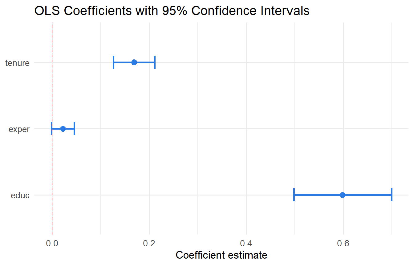
6 The F-Test for Joint Hypotheses
6.1 SSR-Ratio Form
A single \(t\)-test assesses one restriction. To test \(q\) restrictions simultaneously, we compare the fit of the restricted model (imposing \(H_0\)) to the unrestricted model. If imposing \(H_0\) makes the fit much worse (SSR increases substantially), we reject \(H_0\).
\[\boxed{F = \frac{(SSR_r - SSR_{ur})/q}{SSR_{ur}/(n-k-1)} \sim F(q,\, n-k-1) \text{ under } H_0}\]
Intuition: The numerator measures the average loss of fit per restriction. The denominator estimates \(\sigma^2\). Their ratio is \(F(q, n-k-1)\) under \(H_0\) because numerator and denominator are independent \(\chi^2\) variates scaled by their degrees of freedom.
6.2 \(R^2\) Form
Since \(SSR = SST(1 - R^2)\) in both models:
\[F = \frac{(SSR_r - SSR_{ur})/q}{SSR_{ur}/(n-k-1)} = \frac{(R^2_{ur} - R^2_r)/q}{(1 - R^2_{ur})/(n-k-1)}\]
This form is especially convenient when the restricted model is the intercept-only model (\(R^2_r = 0\)), giving the overall \(F\)-statistic:
\[F_{overall} = \frac{R^2/k}{(1-R^2)/(n-k-1)}\]
6.3 Worked Example: Hand-Calculated F-Test
Suppose we want to test whether exper and tenure jointly matter, controlling for educ.
# Unrestricted: wage ~ educ + exper + tenure
fit_ur <- lm(wage ~ educ + exper + tenure, data = wage1)

# Restricted: impose beta_exper = beta_tenure = 0
fit_r  <- lm(wage ~ educ, data = wage1)

SSR_ur <- sum(resid(fit_ur)^2)
SSR_r  <- sum(resid(fit_r)^2)
n      <- nrow(wage1)
k      <- 3   # unrestricted model parameters (excl. intercept)
q      <- 2   # number of restrictions

F_stat <- ((SSR_r - SSR_ur) / q) / (SSR_ur / (n - k - 1))

cat("SSR (restricted):  ", round(SSR_r,  2), "\n")
SSR (restricted): 5981 cat("SSR (unrestricted):", round(SSR_ur, 2), "\n")SSR (unrestricted): 4966 cat("F-statistic (hand):", round(F_stat, 4), "\n")F-statistic (hand): 53.31 cat("Critical value (5%):", round(qf(0.95, q, n - k - 1), 4), "\n")Critical value (5%): 3.013 cat("p-value: ", round(pf(F_stat, q, n - k - 1, lower.tail = FALSE), 6), "\n")p-value: 0 # Verify with linearHypothesis
linearHypothesis(fit_ur, c("exper = 0", "tenure = 0"))Both approaches give the same \(F\)-statistic. Since \(F > F_{crit}\), we reject \(H_0\) at the 5% level: experience and tenure jointly matter.
6.4 Overall Significance
glance(fit) |> dplyr::select(r.squared, statistic, p.value, df, df.residual)The overall \(F\)-statistic tests whether all regressors are jointly zero. Verify the \(R^2\)-form:
R2 <- glance(fit)$r.squared
k_vars <- 3
n <- nrow(wage1)
F_r2_form <- (R2 / k_vars) / ((1 - R2) / (n - k_vars - 1))
cat("F from R^2 form:", round(F_r2_form, 4), "\n")
F from R^2 form: 76.87 cat("F from summary: ", round(glance(fit)$statistic, 4), "\n")F from summary: 76.87 7 The Reparameterisation Trick
The standard \(t\)-test handles \(H_0: \beta_j = 0\) directly. For non-zero null hypotheses or hypotheses about linear combinations of coefficients, the reparameterisation trick rewrites the model so the restriction of interest is simply “does the new coefficient equal zero?”.
7.1 Non-Zero Null Hypothesis
Test \(H_0: \beta_{educ} = 1\) (return to education is exactly $1/hour). Simply compute:
\[t = \frac{\hat{\beta}_{educ} - 1}{\text{se}(\hat{\beta}_{educ})}\]
No reparameterisation needed — this is just the shifted \(t\)-statistic.
b_educ  <- coef(fit)["educ"]
se_educ <- tidy(fit) |> dplyr::filter(term == "educ") |> dplyr::pull(std.error)
t_1     <- (b_educ - 1) / se_educ
p_two   <- 2 * pt(-abs(t_1), df = n - k - 1)
cat("t-stat:", round(t_1, 3), "  p-value:", round(p_two, 4), "\n")
t-stat: -7.82 p-value: 0 7.2 Linear Combination via Reparameterisation
Consider testing \(H_0: \beta_{exper} = 2\beta_{tenure}\) (the return to experience is twice the return to tenure).
Step 1. Define \(\theta = \beta_{exper} - 2\beta_{tenure}\); we test \(H_0: \theta = 0\).
Step 2. Reparameterise: let \(\beta_{exper} = \theta + 2\beta_{tenure}\). Substitute into the model:
\[\text{wage} = \beta_0 + \beta_{educ}\,\text{educ} + (\theta + 2\beta_{tenure})\,\text{exper} + \beta_{tenure}\,\text{tenure} + u\] \[= \beta_0 + \beta_{educ}\,\text{educ} + \theta\,\text{exper} + \beta_{tenure}(\text{tenure} + 2\,\text{exper}) + u\]
Step 3. Create the composite variable \(z = \text{tenure} + 2 \cdot \text{exper}\) and regress wage on educ, exper, and z. The coefficient on exper in this new regression is \(\theta\), and its \(t\)-test directly tests \(H_0: \theta = 0\).
wage1_rp <- wage1 |> mutate(z = tenure + 2 * exper)
fit_rp   <- lm(wage ~ educ + exper + z, data = wage1_rp)

# theta = coefficient on exper in reparameterised model
tidy(fit_rp) |> dplyr::filter(term == "exper")
# Verify with linearHypothesis — should give same p-value
linearHypothesis(fit, "exper = 2 * tenure")The p-value matches — both approaches test the same restriction. The reparameterisation trick is especially useful for constructing confidence intervals for \(\theta\): the CI from confint() on the reparameterised regression is automatically the CI for \(\beta_{exper} - 2\beta_{tenure}\).
7.3 One-Sided Tests
For \(H_0: \beta_{educ} = 0\) vs. \(H_1: \beta_{educ} > 0\) (education raises wages):
t_stat <- tidy(fit) |> dplyr::filter(term == "educ") |> dplyr::pull(statistic)
p_one  <- pt(t_stat, df = n - k - 1, lower.tail = FALSE)
cat("One-sided p-value:", round(p_one, 6), "\n")
One-sided p-value: 0 The one-sided p-value is half the two-sided p-value when \(t > 0\) and the alternative is \(H_1: \beta > 0\).
8 The Relationship Between t, F, and CI
For a single restriction:
\[F = t^2 \qquad (q = 1)\]
Rejecting the \(F\)-test at the 5% level with one restriction is identical to: (i) rejecting the two-sided \(t\)-test at 5%, and (ii) the 95% CI not containing the null value.
All three representations carry the same information for a single coefficient. Only \(F\) generalises to multiple restrictions — this is why we use it for joint tests.
9 Testing Economic Hypotheses
Economic theory often implies specific parameter restrictions, not just zero tests.
Example 1: Does an extra year of experience have the same wage effect as an extra year of tenure?
\[H_0: \beta_{exper} = \beta_{tenure} \quad \text{vs.} \quad H_1: \beta_{exper} \neq \beta_{tenure}\]
linearHypothesis(fit, "exper = tenure")Example 2: Is the return to education at least $1 per hour?
\[H_0: \beta_{educ} \leq 1 \quad \text{vs.} \quad H_1: \beta_{educ} > 1\]
This is a one-sided test with the shifted statistic. We computed this above.
10 Tutorials
Tutorial 5.1 Using the regression wage ~ educ + exper + tenure:
- Manually compute the \(t\)-statistic for
educand verify it matchestidy(). - Construct a 99% confidence interval for \(\beta_{educ}\) manually and compare to the 95% CI.
- Apply the six-step protocol to test \(H_0: \beta_{educ} = 0.5\) against \(H_1: \beta_{educ} \neq 0.5\) at the 1% level.
TipSolution
result  <- tidy(fit, conf.int = TRUE) |> dplyr::filter(term == "educ")
b_educ  <- result$estimate
se_educ <- result$std.error
df_res  <- n - k - 1

# a) t-statistic
cat("t-stat (manual):", round(b_educ / se_educ, 4), "\n")
t-stat (manual): 11.68 cat("t-stat (tidy): ", round(result$statistic, 4), "\n\n")t-stat (tidy): 11.68 # b) 99% CI
ci_99 <- b_educ + qt(c(0.005, 0.995), df = df_res) * se_educ
cat("95% CI: [", round(result$conf.low, 3), ",", round(result$conf.high, 3), "]\n")95% CI: [ 0.498 , 0.7 ]cat("99% CI: [", round(ci_99[1], 3), ",", round(ci_99[2], 3), "]\n\n")99% CI: [ 0.466 , 0.732 ]# c) Six-step protocol
# 1. H0: beta_educ = 0.5; H1: beta_educ != 0.5
# 2. t = (b_educ - 0.5)/se_educ ~ t(n-k-1) under H0
# 3. alpha = 0.01
# 4. Reject if |t| > t_0.005,df
crit <- qt(0.995, df = df_res)
t_05 <- (b_educ - 0.5) / se_educ
p_05 <- 2 * pt(-abs(t_05), df = df_res)
cat("Step 4 critical value:", round(crit, 3), "\n")Step 4 critical value: 2.585 cat("Step 5 t-statistic: ", round(t_05, 4), "\n")Step 5 t-statistic: 1.93 cat("Step 5 p-value: ", round(p_05, 6), "\n")Step 5 p-value: 0.05418 cat("Step 6: |t| =", round(abs(t_05), 2), ">", round(crit, 2),
"— reject H0 at 1% level.\n")Step 6: |t| = 1.93 > 2.59 — reject H0 at 1% level.Tutorial 5.2 Explain why multiple individual \(t\)-tests cannot substitute for an \(F\)-test when testing joint significance. Verify with a simulation: generate data where \(\beta_1 = \beta_2 = 0\), run 5,000 regressions, and record how often at least one coefficient is significant at 5%.
TipSolution
set.seed(1)

results_mult <- map_lgl(1:5000, function(i) {
  x1 <- rnorm(100); x2 <- rnorm(100)
  y  <- rnorm(100)
  p  <- tidy(lm(y ~ x1 + x2))$p.value[-1]
  any(p < 0.05)
})

cat("Simulated type I error rate:", round(mean(results_mult), 3), "\n")
Simulated type I error rate: 0.094 cat("Theoretical (1-(0.95)^2): ", round(1 - 0.95^2, 3), "\n")Theoretical (1-(0.95)^2): 0.098 With two independent 5% tests, the probability of at least one false positive is approximately \(1 - (1-0.05)^2 \approx 9.75\%\) — nearly double the nominal level. The \(F\)-test controls the joint significance level at exactly \(\alpha = 5\%\).
Tutorial 5.3 Using wooldridge::gpa1, regress colGPA on hsGPA, ACT, and skipped.
- Apply the six-step protocol to test joint significance of
hsGPAandACT(i.e., \(H_0: \beta_{hsGPA} = \beta_{ACT} = 0\)) at the 5% level. - Compute the \(F\)-statistic by hand using the SSR formula and verify it matches
linearHypothesis(). - Use the reparameterisation trick to test \(H_0: \beta_{hsGPA} = 3\beta_{ACT}\) and construct a 95% CI for \(\beta_{hsGPA} - 3\beta_{ACT}\).
TipSolution
data("gpa1", package = "wooldridge")
fit_gpa  <- lm(colGPA ~ hsGPA + ACT + skipped, data = gpa1)
fit_gpa_r <- lm(colGPA ~ skipped, data = gpa1)

n_gpa <- nrow(gpa1); k_gpa <- 3; q_gpa <- 2

# a) Six-step protocol
SSR_ur_gpa <- sum(resid(fit_gpa)^2)
SSR_r_gpa  <- sum(resid(fit_gpa_r)^2)
F_hand     <- ((SSR_r_gpa - SSR_ur_gpa)/q_gpa) / (SSR_ur_gpa/(n_gpa - k_gpa - 1))
crit_gpa   <- qf(0.95, q_gpa, n_gpa - k_gpa - 1)

cat("F-statistic (hand):", round(F_hand, 4), "\n")
F-statistic (hand): 14.75 cat("Critical value: ", round(crit_gpa, 4), "\n")Critical value: 3.062 cat("Conclusion: F =", round(F_hand,2), ">", round(crit_gpa,2),
"— reject H0 at 5%.\n\n")Conclusion: F = 14.75 > 3.06 — reject H0 at 5%.# b) Verify with linearHypothesis
linearHypothesis(fit_gpa, c("hsGPA = 0", "ACT = 0"))# c) Reparameterise: theta = beta_hsGPA - 3*beta_ACT
gpa1_rp <- gpa1 |> mutate(z = ACT * 3 + hsGPA)
# Substitute beta_hsGPA = theta + 3*beta_ACT
# colGPA = b0 + (theta + 3*b_ACT)*hsGPA + b_ACT*ACT + b_skip*skipped
# = b0 + theta*hsGPA + b_ACT*(3*hsGPA + ACT) + b_skip*skipped
gpa1_rp2 <- gpa1 |> mutate(z = 3 * hsGPA + ACT)
fit_rp <- lm(colGPA ~ hsGPA + z + skipped, data = gpa1_rp2)
tidy(fit_rp, conf.int = TRUE) |> dplyr::filter(term == "hsGPA")The coefficient on hsGPA in the reparameterised model is \(\hat{\theta} = \hat{\beta}_{hsGPA} - 3\hat{\beta}_{ACT}\), and its confidence interval is the CI for this linear combination.