---
title: "Chapter 10: Serial Correlation"
subtitle: "Autocorrelation in time series: detection and HAC inference"
---
```{r}
#| label: setup
#| include: false
library(tidyverse)
library(broom)
library(modelsummary)
library(lmtest)
library(sandwich)
library(wooldridge)
theme_set(theme_minimal(base_size = 13))
options(digits = 4, scipen = 999)
data("phillips", package = "wooldridge")
data("intdef", package = "wooldridge")
```
::: {.callout-note}
## Learning Objectives
By the end of this chapter you will be able to:
- Define serial (auto)correlation and explain why it arises in time-series regressions
- Interpret ACF and PACF plots to diagnose autocorrelation
- Apply the Durbin-Watson and Breusch-Godfrey tests
- Explain why OLS SEs are invalid under serial correlation and what the consequences are
- Compute Newey-West HAC standard errors using `sandwich::NeweyWest()`
- Describe the FGLS/Cochrane-Orcutt correction as an efficiency improvement
:::
---
## What Is Serial Correlation?
In time-series data, regression errors are often **correlated across time**. This violates the independence assumption underlying standard OLS inference.
The simplest model is **AR(1) errors**:
$$
u_t = \rho u_{t-1} + e_t, \quad e_t \sim \text{i.i.d.}(0, \sigma_e^2), \quad |\rho| < 1
$$
- $\rho > 0$: **positive serial correlation** — common in economics (errors persist)
- $\rho < 0$: negative serial correlation — less common, often mechanical
- $\rho = 0$: no serial correlation (the null hypothesis we test)
### Why Does It Arise?
Serial correlation typically occurs because:
1. **Omitted variables** that are autocorrelated (e.g., missing a lagged variable)
2. **Model misspecification** (wrong functional form or dynamics)
3. **Inherently persistent** economic processes (business cycles, trends)
### Consequences
Like heteroskedasticity, serial correlation:
- Does **not** bias OLS coefficient estimates (if the model is correctly specified)
- **Does** bias the standard error formula — typically **downward** (SEs too small)
- Makes t-tests and F-tests **anti-conservative**: we reject $H_0$ too often
---
## Visualising Autocorrelation
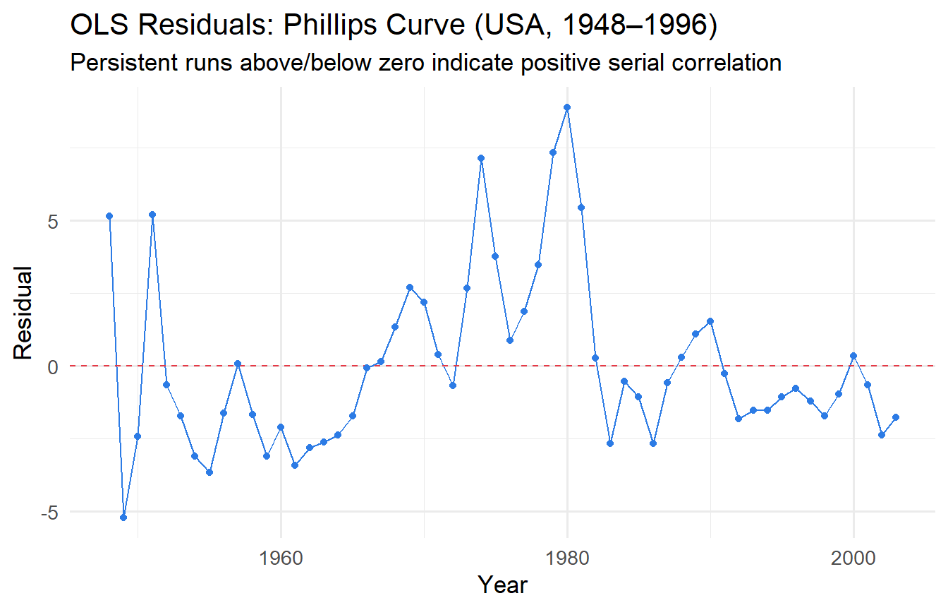
### Residual Time-Series Plot
```{r}
#| label: fig-resid-time
#| fig-cap: "OLS residuals over time: persistent pattern suggests positive serial correlation."
fit_phillips <- lm(inf ~ unem, data = phillips)

augment(fit_phillips) |>
  mutate(year = phillips$year) |>
  ggplot(aes(year, .resid)) +
  geom_line(colour = "#2c7be5") +
  geom_hline(yintercept = 0, linetype = "dashed", colour = "#e63946") +
  geom_point(size = 1.5, colour = "#2c7be5") +
  labs(x = "Year", y = "Residual",
       title = "OLS Residuals: Phillips Curve (USA, 1948–1996)",
       subtitle = "Persistent runs above/below zero indicate positive serial correlation")
```
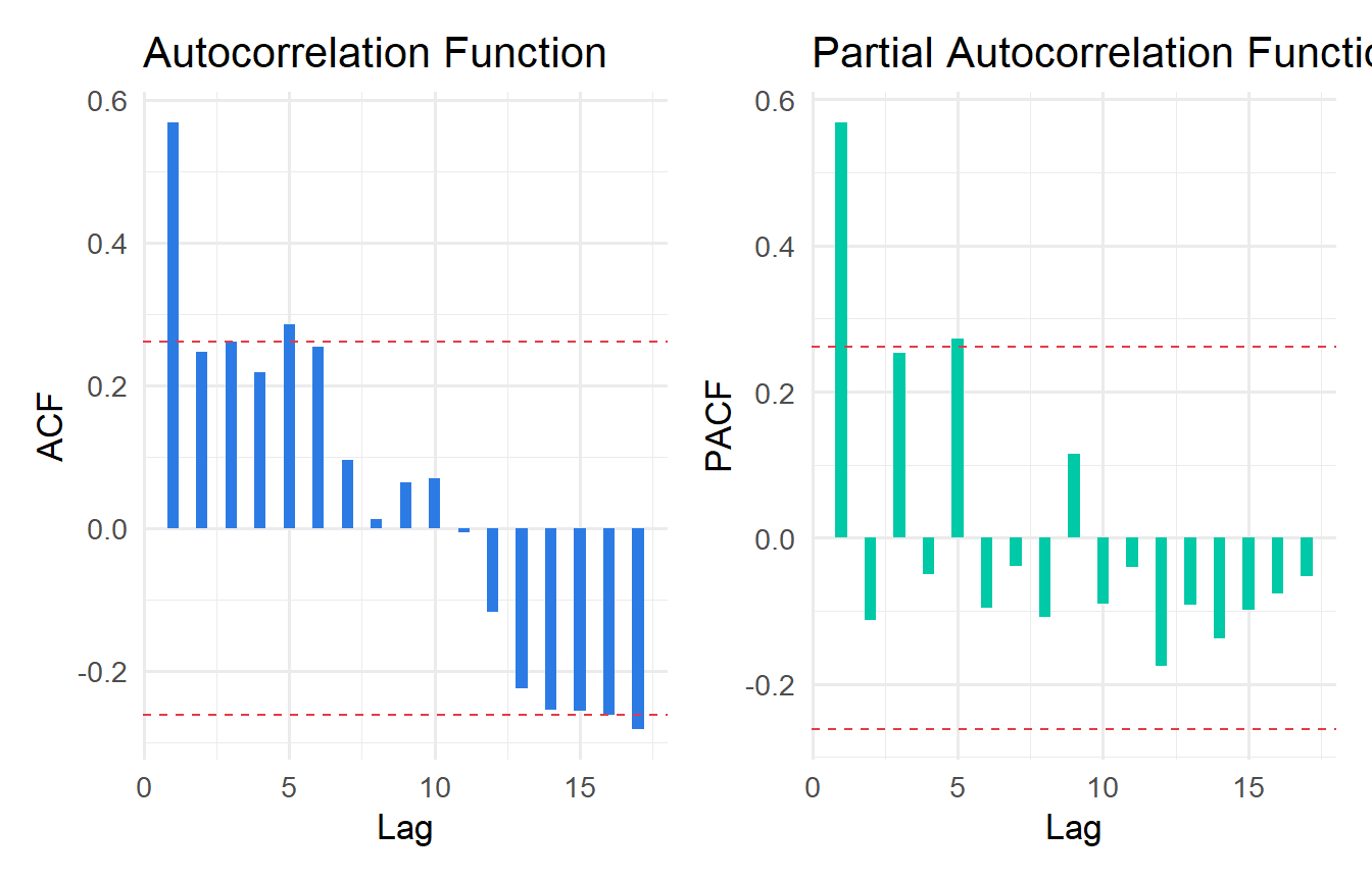
### ACF and PACF Plots
The **autocorrelation function (ACF)** and **partial autocorrelation function (PACF)** are the standard tools for diagnosing serial correlation.
```{r}
#| label: fig-acf-pacf
#| fig-cap: "ACF and PACF of OLS residuals. Significant spikes indicate autocorrelation."
resids <- residuals(fit_phillips)

# ACF
acf_data <- acf(resids, plot = FALSE)
pacf_data <- pacf(resids, plot = FALSE)

ci_bound <- qnorm(0.975) / sqrt(length(resids))

p_acf <- tibble(
  lag  = acf_data$lag[-1],
  acf  = acf_data$acf[-1]
) |>
  ggplot(aes(lag, acf)) +
  geom_col(fill = "#2c7be5", width = 0.4) +
  geom_hline(yintercept = c(ci_bound, -ci_bound),
             linetype = "dashed", colour = "#e63946") +
  labs(x = "Lag", y = "ACF", title = "Autocorrelation Function")

p_pacf <- tibble(
  lag  = pacf_data$lag,
  pacf = pacf_data$acf
) |>
  ggplot(aes(lag, pacf)) +
  geom_col(fill = "#00c9a7", width = 0.4) +
  geom_hline(yintercept = c(ci_bound, -ci_bound),
             linetype = "dashed", colour = "#e63946") +
  labs(x = "Lag", y = "PACF", title = "Partial Autocorrelation Function")

library(patchwork)
p_acf + p_pacf
```
**Reading ACF/PACF:** Bars exceeding the dashed 95% confidence bands (approximately $\pm 1.96/\sqrt{T}$) indicate statistically significant autocorrelation at that lag. A gradually decaying ACF with a single significant spike in the PACF at lag 1 is the signature of AR(1) errors.
---
## Formal Tests for Serial Correlation
### Durbin-Watson Test
The **Durbin-Watson (DW) statistic** tests $H_0: \rho = 0$ against $H_1: \rho > 0$:
$$
DW = \frac{\sum_{t=2}^T (\hat{u}_t - \hat{u}_{t-1})^2}{\sum_{t=1}^T \hat{u}_t^2} \approx 2(1 - \hat{\rho})
$$
- DW ≈ 2: no serial correlation
- DW < 2: positive serial correlation ($\hat{\rho} > 0$)
- DW > 2: negative serial correlation ($\hat{\rho} < 0$)
```{r}
#| label: dw-test
dwtest(fit_phillips)
```
::: {.callout-important}
## Limitations of the DW Test
- Only tests AR(1) — misses higher-order autocorrelation
- Cannot be used with **lagged dependent variables** as regressors (use BG test instead)
- Has an inconclusive region — the exact critical values depend on the regressors
:::
### Breusch-Godfrey Test
The **Breusch-Godfrey (BG) test** is more general: it tests for AR($p$) serial correlation and is valid even with lagged dependent variables.
```{r}
#| label: bg-test
# Test for AR(1) serial correlation
bgtest(fit_phillips, order = 1)
# Test for up to AR(4) serial correlation
bgtest(fit_phillips, order = 4)
```
Both tests strongly reject the null of no serial correlation in the Phillips curve regression — not surprising given the persistent residual pattern we observed.
---
## The Solution: Newey-West HAC Standard Errors
Just as robust SEs solve the heteroskedasticity problem, **HAC (heteroskedasticity and autocorrelation consistent) standard errors** — also called **Newey-West standard errors** — solve the serial correlation problem.
The HAC variance estimator accounts for both heteroskedasticity and autocorrelation by including weighted cross-products of residuals at nearby time periods:
$$
\widehat{\text{Var}}_{\text{HAC}}(\hat{\boldsymbol{\beta}}) = (X'X)^{-1} \hat{S} (X'X)^{-1}
$$
where $\hat{S}$ sums up to $L$ lags of weighted autocovariances. The **bandwidth** $L$ is typically chosen as $\lfloor 4(T/100)^{2/9} \rfloor$ or similar rule.
```{r}
#| label: hac-se
# OLS with conventional SEs
coeftest(fit_phillips)
# OLS with Newey-West HAC SEs
coeftest(fit_phillips, vcov = NeweyWest(fit_phillips))
```
```{r}
#| label: hac-comparison
#| tbl-cap: "Conventional vs. HAC standard errors for the Phillips curve."
# Build comparison using modelsummary with custom vcov
modelsummary(
  list(
    "OLS (conventional)" = fit_phillips,
    "OLS (Newey-West HAC)" = fit_phillips
  ),
  vcov = list("iid", NeweyWest),
  stars   = TRUE,
  gof_map = c("nobs", "r.squared"),
  title   = "Phillips Curve: Conventional vs. HAC Standard Errors"
)
```
With HAC standard errors, the standard error on `unem` increases substantially — reflecting the uncertainty that serial correlation adds. This is why conventional SEs in time-series regressions are anti-conservative.
::: {.callout-tip}
## Choosing the HAC Bandwidth
The `NeweyWest()` function selects the bandwidth automatically using a data-driven procedure. You can also specify it manually:
```r
NeweyWest(fit, lag = 4, prewhite = FALSE)
```
For annual data, lags of 2–4 are common. For quarterly data, 4–8 lags. For monthly data, 12+ lags. When in doubt, use the automatic selection.
:::
---
## FGLS: Correcting for AR(1) Errors
If you believe errors follow an AR(1) process, **Feasible GLS (FGLS)** — also called the **Cochrane-Orcutt** procedure — can produce more efficient estimates:
1. Estimate OLS and obtain residuals $\hat{u}_t$
2. Estimate $\hat{\rho}$ from $\hat{u}_t = \rho \hat{u}_{t-1} + e_t$
3. **Quasi-difference** the data: $\tilde{y}_t = y_t - \hat{\rho} y_{t-1}$, $\tilde{x}_t = x_t - \hat{\rho} x_{t-1}$
4. Run OLS on the quasi-differenced data
```{r}
#| label: fgls-ar1
# Step 2: estimate rho
rho_hat <- coef(lm(residuals(fit_phillips)[-1] ~
                     residuals(fit_phillips)[-nrow(phillips)] - 1))
cat("Estimated rho:", round(rho_hat, 4), "\n")
# Step 3-4: quasi-difference and re-estimate
T_n <- nrow(phillips)
phillips_qd <- phillips |>
  mutate(
    inf_qd  = inf  - rho_hat * lag(inf),
    unem_qd = unem - rho_hat * lag(unem)
  ) |>
  drop_na()

fit_fgls <- lm(inf_qd ~ unem_qd, data = phillips_qd)

modelsummary(
  list("OLS" = fit_phillips, "FGLS (Cochrane-Orcutt)" = fit_fgls),
  stars   = TRUE,
  gof_map = c("nobs", "r.squared"),
  title   = "Phillips Curve: OLS vs. FGLS"
)
```
::: {.callout-tip}
## OLS + HAC vs. FGLS
- **OLS + HAC SEs**: Correct for invalid inference but do not improve efficiency. Requires no assumptions about the form of serial correlation.
- **FGLS**: More efficient (lower variance) if the AR(1) assumption is correct. But misspecifying the error process leads to inconsistency.
In modern applied work, **OLS + HAC SEs** is the dominant approach, used in the vast majority of published time-series papers. FGLS is less common because misspecification risk is high.
:::
---
## Tutorials
**Tutorial 10.1**
Using `wooldridge::intdef` (interest rates and budget deficits, USA):
a. Regress `i3` (3-month T-bill rate) on `inf` (inflation) and `def` (budget deficit as % of GDP).
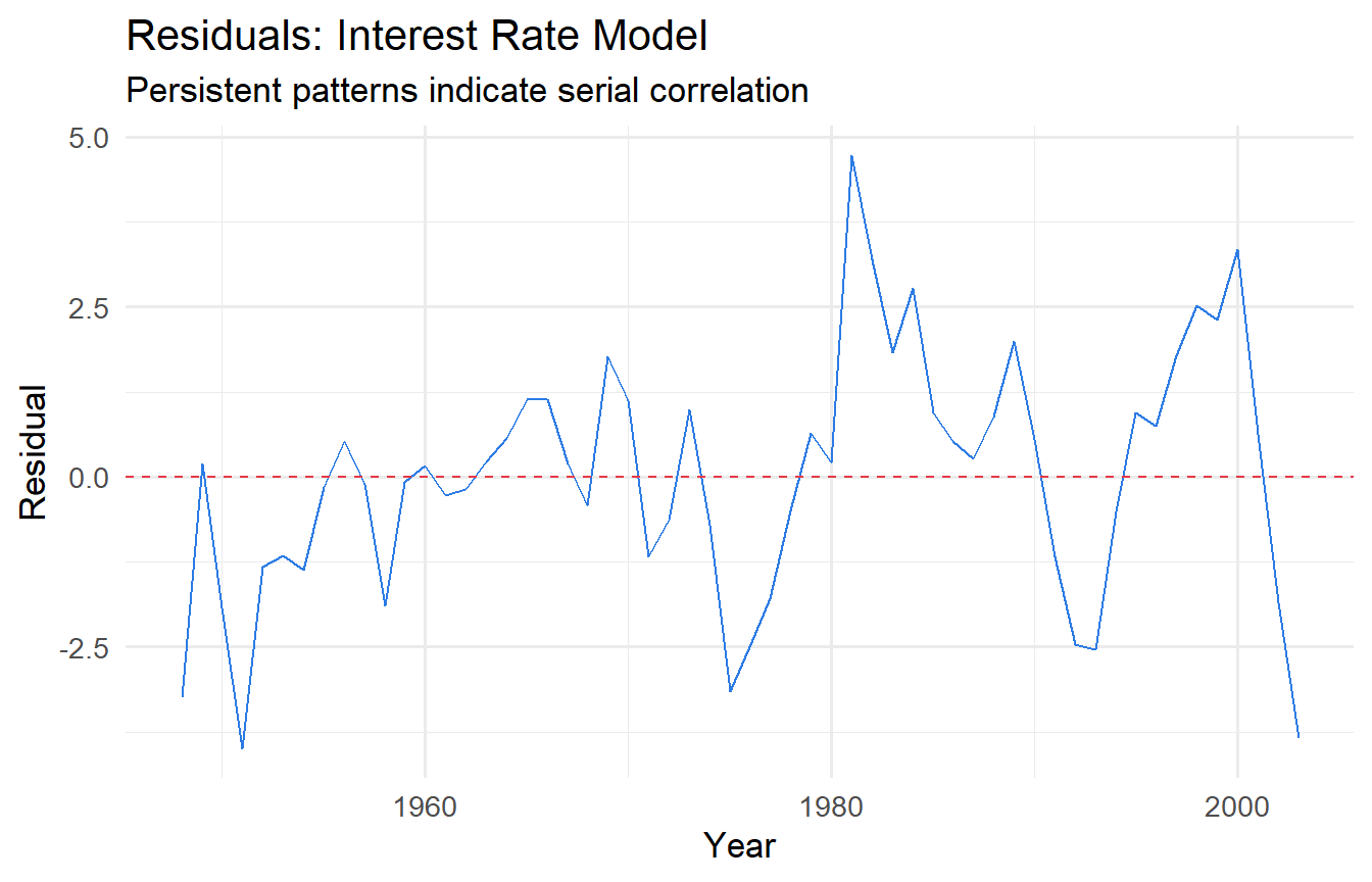
b. Plot the residuals over time. Does the pattern suggest serial correlation?
c. Apply the DW test and the BG test (up to order 2). What do you conclude?
::: {.callout-tip collapse="true"}
## Solution
```{r}
#| label: ex10-1
fit_intdef <- lm(i3 ~ inf + def, data = intdef)

# b) Residuals over time
augment(fit_intdef) |>
  mutate(year = intdef$year) |>
  ggplot(aes(year, .resid)) +
  geom_line(colour = "#2c7be5") +
  geom_hline(yintercept = 0, linetype = "dashed", colour = "#e63946") +
  labs(x = "Year", y = "Residual",
       title = "Residuals: Interest Rate Model",
       subtitle = "Persistent patterns indicate serial correlation")
# c) Tests
dwtest(fit_intdef)
bgtest(fit_intdef, order = 2)
```
The residual plot typically shows persistent runs — positive residuals followed by positive residuals. Both the DW and BG tests should reject the null of no serial correlation. This indicates the static model is misspecified — a dynamic model with lagged interest rates would likely fit better (Chapter 11).
:::
**Tutorial 10.2**
Using the same `intdef` dataset, compare OLS with conventional SEs vs. Newey-West HAC SEs. Focus on the inference for `def` (budget deficit). Does the statistical significance of the budget deficit change?
::: {.callout-tip collapse="true"}
## Solution
```{r}
#| label: ex10-2
coeftest(fit_intdef)
coeftest(fit_intdef, vcov = NeweyWest(fit_intdef))
modelsummary(
  list(
    "OLS (conventional)" = fit_intdef,
    "OLS (Newey-West)"   = fit_intdef
  ),
  vcov    = list("iid", NeweyWest),
  stars   = TRUE,
  gof_map = c("nobs", "r.squared"),
  title   = "Interest Rate Model: Conventional vs. HAC SEs"
)
```
The HAC SEs will typically be larger than conventional SEs. Check whether the t-statistic for `def` crosses the critical threshold — in some specifications, the deficit becomes insignificant once valid SEs are used, raising doubts about a mechanical link between deficits and interest rates (the "crowding out" hypothesis).
:::
**Tutorial 10.3**
Simulate an AR(1) process with $\rho = 0.8$ and show the consequences of ignoring serial correlation. Generate $T = 100$ observations with $y_t = 1 + 0.5 x_t + u_t$ where $u_t = 0.8 u_{t-1} + e_t$. Over 2,000 replications, compare the rejection rate of the $t$-test on $\beta_1$ using conventional vs. Newey-West SEs (true $H_0$ holds, i.e., test $\beta_1 = 0.5$).
::: {.callout-tip collapse="true"}
## Solution
```{r}
#| label: ex10-3
set.seed(42)
T_obs  <- 100
rho    <- 0.8
n_sims <- 2000

results_sc <- map_dfr(1:n_sims, function(i) {
  x   <- rnorm(T_obs)
  e   <- rnorm(T_obs)
  u   <- numeric(T_obs)
  u[1] <- e[1]
  for (t in 2:T_obs) u[t] <- rho * u[t - 1] + e[t]
  y <- 1 + 0.5 * x + u
  fit <- lm(y ~ x)

  # Conventional t-test
  t_conv <- (coef(fit)[2] - 0.5) / sqrt(diag(vcov(fit)))[2]
  p_conv <- 2 * pt(-abs(t_conv), df = T_obs - 2)

  # HAC t-test
  se_hac  <- sqrt(diag(NeweyWest(fit)))[2]
  t_hac   <- (coef(fit)[2] - 0.5) / se_hac
  p_hac   <- 2 * pt(-abs(t_hac), df = T_obs - 2)

  tibble(reject_conv = p_conv < 0.05, reject_hac = p_hac < 0.05)
})

cat("Rejection rate (conventional SEs):", round(mean(results_sc$reject_conv), 3), "\n")
cat("Rejection rate (Newey-West HAC): ", round(mean(results_sc$reject_hac), 3), "\n")
cat("Nominal level: 0.05\n")
```
With conventional SEs, the rejection rate is far above 5% — the test is badly over-sized. With Newey-West HAC SEs, the rejection rate is close to the nominal 5% level, confirming that HAC inference is approximately valid even under strong serial correlation.
:::