---
title: "Chapter 4: Properties of OLS — BLUE and Gauss-Markov"
subtitle: "Why OLS works, when it works, and simulation-based intuition"
---
```{r}
#| label: setup
#| include: false
library(tidyverse)
library(broom)
library(patchwork)
library(wooldridge)
theme_set(theme_minimal(base_size = 13))
options(digits = 4, scipen = 999)
set.seed(42)
```
::: {.callout-note}
## Learning Objectives
By the end of this chapter you will be able to:
- State the CLM assumptions in both scalar and matrix notation
- Distinguish an **estimator** (a rule) from an **estimate** (a number)
- Prove OLS unbiasedness algebraically in both scalar and matrix form
- Derive $\text{Var}(\hat{\boldsymbol{\beta}} \mid \mathbf{X}) = \sigma^2 (\mathbf{X}'\mathbf{X})^{-1}$
- State and apply the Gauss-Markov theorem
- Derive the omitted variable bias formula algebraically
- Explain how rescaling $x$ or $y$ affects OLS estimates
- Use Monte Carlo simulation to verify unbiasedness and efficiency in R
:::
---
## Estimator vs. Estimate
A common source of confusion is the distinction between an **estimator** and an **estimate**.
An **estimator** is a *function* of the data — a rule or formula that, when applied to any sample, produces a number. Before we collect data, the estimator is a random variable with its own distribution (the **sampling distribution**). The OLS slope
$$\hat{\beta}_1 = \frac{\sum_{i=1}^n (x_i - \bar{x})(y_i - \bar{y})}{\sum_{i=1}^n (x_i - \bar{x})^2}$$
is an estimator: it varies from sample to sample because it depends on the random $y_i$ (which in turn depend on the random errors $u_i$).
An **estimate** is the specific number you obtain after plugging in a particular realised sample. If your data give $\hat{\beta}_1 = 2.34$, that is the estimate for this dataset. It is a fixed number, not a random variable.
This distinction matters for inference. Unbiasedness, variance, and confidence intervals are properties of the *estimator* (averaged over hypothetical repeated samples), not of any single *estimate*.
---
## The Classical Linear Model Assumptions
### Scalar (Simple Regression) Form
| Label | Assumption | Statement |
|---|---|---|
| SLR.1 | Linearity in parameters | $y = \beta_0 + \beta_1 x + u$ |
| SLR.2 | Random sampling | $(x_i, y_i)$ i.i.d. from the population |
| SLR.3 | No perfect collinearity | $\text{Var}(x) > 0$ (not all $x_i$ identical) |
| SLR.4 | Zero conditional mean | $E[u \mid x] = 0$ |
| SLR.5 | Homoskedasticity | $\text{Var}(u \mid x) = \sigma^2$ (constant) |
| SLR.6 | Normality | $u \mid x \sim \mathcal{N}(0, \sigma^2)$ |
SLR.1–4 deliver **unbiasedness**. Adding SLR.5 delivers **BLUE** (minimum variance among linear unbiased estimators). Adding SLR.6 delivers exact finite-sample inference via the $t$ and $F$ distributions.
### Matrix (Multiple Regression) Form
Stack observations: $\mathbf{y} = \mathbf{X}\boldsymbol{\beta} + \mathbf{u}$, where $\mathbf{y}$ is $n \times 1$, $\mathbf{X}$ is $n \times (k+1)$ with a leading column of ones, $\boldsymbol{\beta}$ is $(k+1) \times 1$, and $\mathbf{u}$ is $n \times 1$.
| Label | Assumption | Matrix Statement |
|---|---|---|
| MLR.1 | Linearity | $\mathbf{y} = \mathbf{X}\boldsymbol{\beta} + \mathbf{u}$ |
| MLR.2 | Random sampling | Rows $(x_i', y_i)$ are i.i.d. |
| MLR.3 | Full column rank | $\text{rank}(\mathbf{X}) = k + 1$ (no perfect multicollinearity) |
| MLR.4 | Zero conditional mean | $E[\mathbf{u} \mid \mathbf{X}] = \mathbf{0}$ |
| MLR.5 | Scalar covariance | $\text{Var}(\mathbf{u} \mid \mathbf{X}) = \sigma^2 \mathbf{I}_n$ |
| MLR.6 | Normality | $\mathbf{u} \mid \mathbf{X} \sim \mathcal{N}(\mathbf{0}, \sigma^2 \mathbf{I}_n)$ |
MLR.5 encodes two conditions simultaneously: (i) each error has variance $\sigma^2$ (homoskedasticity) and (ii) errors are uncorrelated across observations (no serial correlation). Both conditions appear in the single matrix equation $\text{Var}(\mathbf{u} \mid \mathbf{X}) = \sigma^2 \mathbf{I}_n$.
---
## Unbiasedness of OLS
### Scalar Proof
Write $\hat{\beta}_1$ in terms of the true data-generating process. From Chapter 3:
$$\hat{\beta}_1 = \frac{\sum(x_i - \bar{x})y_i}{\sum(x_i - \bar{x})^2}$$
Substituting $y_i = \beta_0 + \beta_1 x_i + u_i$:
$$\hat{\beta}_1 = \frac{\sum(x_i - \bar{x})(\beta_0 + \beta_1 x_i + u_i)}{\sum(x_i - \bar{x})^2}$$
The $\beta_0$ term vanishes because $\sum(x_i - \bar{x}) = 0$. Therefore:
$$\hat{\beta}_1 = \beta_1 + \frac{\sum(x_i - \bar{x})u_i}{\sum(x_i - \bar{x})^2} = \beta_1 + \sum_{i=1}^n w_i u_i$$
where $w_i = (x_i - \bar{x}) / \sum(x_i - \bar{x})^2$ are fixed constants (conditional on $\mathbf{x}$). Taking conditional expectations:
$$E[\hat{\beta}_1 \mid \mathbf{x}] = \beta_1 + \sum w_i \underbrace{E[u_i \mid \mathbf{x}]}_{=\,0 \text{ by SLR.4}} = \beta_1$$
By the Law of Iterated Expectations, $E[\hat{\beta}_1] = E_{\mathbf{x}}[E[\hat{\beta}_1 \mid \mathbf{x}]] = \beta_1$. $\blacksquare$
### Matrix Proof
Recall from Chapter 3 that $\hat{\boldsymbol{\beta}} = (\mathbf{X}'\mathbf{X})^{-1}\mathbf{X}'\mathbf{y}$. Substitute the true DGP $\mathbf{y} = \mathbf{X}\boldsymbol{\beta} + \mathbf{u}$:
$$\hat{\boldsymbol{\beta}} = (\mathbf{X}'\mathbf{X})^{-1}\mathbf{X}'(\mathbf{X}\boldsymbol{\beta} + \mathbf{u}) = (\mathbf{X}'\mathbf{X})^{-1}\mathbf{X}'\mathbf{X}\boldsymbol{\beta} + (\mathbf{X}'\mathbf{X})^{-1}\mathbf{X}'\mathbf{u}$$
$$\hat{\boldsymbol{\beta}} = \boldsymbol{\beta} + (\mathbf{X}'\mathbf{X})^{-1}\mathbf{X}'\mathbf{u}$$
Taking conditional expectations:
$$E[\hat{\boldsymbol{\beta}} \mid \mathbf{X}] = \boldsymbol{\beta} + (\mathbf{X}'\mathbf{X})^{-1}\mathbf{X}' \underbrace{E[\mathbf{u} \mid \mathbf{X}]}_{=\,\mathbf{0} \text{ by MLR.4}} = \boldsymbol{\beta}$$
By the Law of Iterated Expectations, $E[\hat{\boldsymbol{\beta}}] = \boldsymbol{\beta}$. $\blacksquare$
::: {.callout-important}
## The Linearity Trick
The key step in both proofs is that $\hat{\boldsymbol{\beta}} = \boldsymbol{\beta} + (\mathbf{X}'\mathbf{X})^{-1}\mathbf{X}'\mathbf{u}$ — the estimator equals the truth plus a **linear function of the errors**. This is what makes the expectation easy to take: $E[A\mathbf{u} \mid \mathbf{X}] = A\,E[\mathbf{u} \mid \mathbf{X}] = \mathbf{0}$ whenever $A$ is non-stochastic given $\mathbf{X}$. Unbiasedness fails when $\mathbf{X}$ and $\mathbf{u}$ are correlated (endogeneity), because then $(\mathbf{X}'\mathbf{X})^{-1}\mathbf{X}'\mathbf{u}$ does not have conditional mean zero.
:::
---
## Variance of the OLS Estimator
### Scalar Formula
Under SLR.1–5, using $\hat{\beta}_1 = \beta_1 + \sum w_i u_i$ with $w_i = (x_i - \bar{x}) / SST_x$:
$$\text{Var}(\hat{\beta}_1 \mid \mathbf{x}) = \sum w_i^2\, \text{Var}(u_i \mid \mathbf{x}) = \sigma^2 \sum w_i^2$$
Since $\sum w_i^2 = \sum (x_i - \bar{x})^2 / SST_x^2 = SST_x / SST_x^2 = 1/SST_x$:
$$\boxed{\text{Var}(\hat{\beta}_1 \mid \mathbf{x}) = \frac{\sigma^2}{SST_x}}$$
### Matrix Derivation of $\text{Var}(\hat{\boldsymbol{\beta}} \mid \mathbf{X}) = \sigma^2(\mathbf{X}'\mathbf{X})^{-1}$
From the unbiasedness derivation, the sampling error is $\hat{\boldsymbol{\beta}} - \boldsymbol{\beta} = (\mathbf{X}'\mathbf{X})^{-1}\mathbf{X}'\mathbf{u}$. The variance-covariance matrix of $\hat{\boldsymbol{\beta}}$ is:
$$\text{Var}(\hat{\boldsymbol{\beta}} \mid \mathbf{X}) = E\!\left[(\hat{\boldsymbol{\beta}} - \boldsymbol{\beta})(\hat{\boldsymbol{\beta}} - \boldsymbol{\beta})' \mid \mathbf{X}\right]$$
$$= E\!\left[(\mathbf{X}'\mathbf{X})^{-1}\mathbf{X}'\mathbf{u}\,\mathbf{u}'\mathbf{X}(\mathbf{X}'\mathbf{X})^{-1} \mid \mathbf{X}\right]$$
$$= (\mathbf{X}'\mathbf{X})^{-1}\mathbf{X}'\, \underbrace{E[\mathbf{u}\mathbf{u}' \mid \mathbf{X}]}_{\sigma^2 \mathbf{I}_n \text{ by MLR.5}}\, \mathbf{X}(\mathbf{X}'\mathbf{X})^{-1}$$
$$= \sigma^2(\mathbf{X}'\mathbf{X})^{-1}\underbrace{\mathbf{X}'\mathbf{X}(\mathbf{X}'\mathbf{X})^{-1}}_{\mathbf{I}_{k+1}}$$
$$\boxed{\text{Var}(\hat{\boldsymbol{\beta}} \mid \mathbf{X}) = \sigma^2 (\mathbf{X}'\mathbf{X})^{-1}}$$
The $(j,j)$ diagonal element of $\sigma^2(\mathbf{X}'\mathbf{X})^{-1}$ is $\text{Var}(\hat{\beta}_j \mid \mathbf{X})$; the off-diagonal $(j,\ell)$ element is $\text{Cov}(\hat{\beta}_j, \hat{\beta}_\ell \mid \mathbf{X})$.
### Estimating $\sigma^2$
The population error variance $\sigma^2 = \text{Var}(u_i \mid x_i)$ is unknown and must be estimated. The natural candidate is the average squared residual, but OLS residuals have only $n - (k+1)$ degrees of freedom (we estimated $k+1$ parameters):
$$\hat{\sigma}^2 = \frac{SSR}{n - k - 1} = \frac{\sum_{i=1}^n \hat{u}_i^2}{n - k - 1} = \frac{\mathbf{\hat{u}}'\mathbf{\hat{u}}}{n - k - 1}$$
**This estimator is unbiased**: $E[\hat{\sigma}^2 \mid \mathbf{X}] = \sigma^2$. The proof requires the trace identity $E[\mathbf{\hat{u}}'\mathbf{\hat{u}} \mid \mathbf{X}] = \sigma^2(n - k - 1)$, which follows because $\mathbf{\hat{u}} = \mathbf{M}_X \mathbf{u}$ and $\text{rank}(\mathbf{M}_X) = n - k - 1$.
Plugging $\hat{\sigma}^2$ into $\sigma^2(\mathbf{X}'\mathbf{X})^{-1}$ yields the **estimated variance-covariance matrix** $\widehat{\text{Var}}(\hat{\boldsymbol{\beta}}) = \hat{\sigma}^2(\mathbf{X}'\mathbf{X})^{-1}$. The diagonal square roots are the **standard errors** reported by `lm()`.
**Implications of $\text{Var}(\hat{\beta}_1) = \sigma^2 / SST_x$:**
1. More noise ($\sigma^2 \uparrow$) → less precise estimates
2. More variation in $x$ ($SST_x \uparrow$) → more precise estimates
3. Larger $n$ → $SST_x = \sum(x_i - \bar{x})^2$ grows → estimates improve with data
---
## The Gauss-Markov Theorem
::: {.callout-note}
## Gauss-Markov Theorem
Under MLR.1–5, the OLS estimator $\hat{\boldsymbol{\beta}}$ is the **Best Linear Unbiased Estimator (BLUE)** of $\boldsymbol{\beta}$.
*Linear*: $\tilde{\boldsymbol{\beta}} = \mathbf{C}\mathbf{y}$ for some matrix $\mathbf{C}$ that may depend on $\mathbf{X}$ but not on $\mathbf{y}$.
*Unbiased*: $E[\tilde{\boldsymbol{\beta}} \mid \mathbf{X}] = \boldsymbol{\beta}$.
*Best*: $\text{Var}(\tilde{\boldsymbol{\beta}} \mid \mathbf{X}) - \text{Var}(\hat{\boldsymbol{\beta}} \mid \mathbf{X})$ is positive semi-definite for any alternative linear unbiased $\tilde{\boldsymbol{\beta}}$.
:::
**Proof sketch.** Let $\tilde{\boldsymbol{\beta}} = \mathbf{C}\mathbf{y}$ be any linear unbiased estimator. For unbiasedness, we need $\mathbf{C}\mathbf{X} = \mathbf{I}$. Write $\mathbf{C} = (\mathbf{X}'\mathbf{X})^{-1}\mathbf{X}' + \mathbf{D}$ where $\mathbf{D}\mathbf{X} = \mathbf{0}$ (the unbiasedness constraint forces this). Then:
$$\text{Var}(\tilde{\boldsymbol{\beta}} \mid \mathbf{X}) = \sigma^2 \mathbf{C}\mathbf{C}' = \sigma^2(\mathbf{X}'\mathbf{X})^{-1} + \sigma^2\mathbf{D}\mathbf{D}'$$
Since $\mathbf{D}\mathbf{D}'$ is positive semi-definite, $\text{Var}(\tilde{\boldsymbol{\beta}}) \geq \text{Var}(\hat{\boldsymbol{\beta}})$ in the matrix sense. $\blacksquare$
The theorem is powerful but its scope is limited. "Best" is only among *linear* estimators. Non-linear estimators (e.g., ridge regression) can have lower variance by introducing bias. And "best" requires MLR.5: if errors are heteroskedastic, **Weighted Least Squares** is BLUE, not OLS (Chapter 9).
---
## Omitted Variable Bias
One of the most important consequences of endogeneity in practice is **omitted variable bias (OVB)**: when a relevant variable is excluded from the regression, its effect leaks into the residual and biases the coefficients on included variables.
### The Algebraic Derivation
Suppose the **true** (long) model is:
$$y_i = \beta_0 + \beta_1 x_{1i} + \beta_2 x_{2i} + u_i \quad \text{where } E[u \mid x_1, x_2] = 0 \tag{Long}$$
But the researcher estimates the **short** model, omitting $x_2$:
$$y_i = \tilde{\beta}_0 + \tilde{\beta}_1 x_{1i} + \tilde{u}_i \tag{Short}$$
Let $\delta_1$ be the coefficient from an auxiliary regression of $x_2$ on $x_1$:
$$x_{2i} = \delta_0 + \delta_1 x_{1i} + v_i \tag{Auxiliary}$$
By the Frisch-Waugh theorem, the OLS slope from the short regression can be shown to satisfy:
$$E[\tilde{\beta}_1] = \beta_1 + \beta_2 \delta_1$$
The **omitted variable bias** is therefore:
$$\text{OVB} = \beta_2 \delta_1 = \underbrace{\beta_2}_{\text{effect of }x_2 \text{ on }y} \times \underbrace{\delta_1}_{\text{correlation of }x_1 \text{ with }x_2}$$
The bias is nonzero if and only if both (i) $x_2$ affects $y$ ($\beta_2 \neq 0$) and (ii) $x_1$ and $x_2$ are correlated ($\delta_1 \neq 0$). Either condition alone is insufficient.
### Algebraic Derivation Detail
From the short model, $\tilde{\beta}_1 = \frac{\sum(x_{1i} - \bar{x}_1)y_i}{SST_{x_1}}$. Substitute the long model:
$$\tilde{\beta}_1 = \frac{\sum(x_{1i} - \bar{x}_1)(\beta_0 + \beta_1 x_{1i} + \beta_2 x_{2i} + u_i)}{SST_{x_1}}$$
$$= \beta_1 + \beta_2 \frac{\sum(x_{1i} - \bar{x}_1)(x_{2i} - \bar{x}_2)}{SST_{x_1}} + \frac{\sum(x_{1i} - \bar{x}_1)u_i}{SST_{x_1}}$$
Taking expectations (the last term has mean zero since $u$ is uncorrelated with $x_1$ in the **long** model):
$$E[\tilde{\beta}_1] = \beta_1 + \beta_2 \cdot \underbrace{\frac{\sum(x_{1i} - \bar{x}_1)(x_{2i} - \bar{x}_2)}{SST_{x_1}}}_{\delta_1 \text{ from auxiliary regression}} = \beta_1 + \beta_2 \delta_1$$
### Sign of the Bias
| $\beta_2 > 0$ | $\beta_2 < 0$ | |
|---|---|---|
| $\delta_1 > 0$ | Positive bias: $\tilde{\beta}_1 > \beta_1$ | Negative bias: $\tilde{\beta}_1 < \beta_1$ |
| $\delta_1 < 0$ | Negative bias | Positive bias |
**Example.** Estimating the return to education, omitting ability. If ability raises wages ($\beta_2 > 0$) and is positively correlated with education ($\delta_1 > 0$), then OVB $> 0$: the OLS coefficient on education overstates the causal return, partly picking up the effect of ability.
```{r}
#| label: fig-ovb
#| fig-cap: "OVB illustrated by simulation. The short regression (red) overstates the slope when the omitted variable is positively correlated with x1."
set.seed(123)
n <- 400

# True DGP: y = 1 + 0.5*x1 + 0.8*x2 + u
x1 <- rnorm(n)
x2 <- 0.7 * x1 + rnorm(n, sd = 0.5)   # x2 correlated with x1
u  <- rnorm(n, sd = 0.5)
y  <- 1 + 0.5 * x1 + 0.8 * x2 + u

df <- tibble(y, x1, x2)

long_fit  <- lm(y ~ x1 + x2, data = df)
short_fit <- lm(y ~ x1, data = df)

cat("Long model (true):  beta_1 =", round(coef(long_fit)["x1"], 3), "\n")
cat("Short model (OVB): beta_1 =", round(coef(short_fit)["x1"], 3), "\n")
cat("Auxiliary delta_1 =", round(coef(lm(x2 ~ x1))["x1"], 3), "\n")
cat("Predicted OVB      =",
    round(coef(long_fit)["x2"] * coef(lm(x2 ~ x1))["x1"], 3), "\n")
```
---
## Rescaling and Units of Measurement
OLS estimates change when we rescale variables, but the *predictions* and *fit* are invariant. Understanding exactly how they change is essential for interpreting coefficients correctly.
### Case 1: Scaling $x$ only
Let $x^* = c \cdot x$ (e.g., converting metres to centimetres, $c = 100$). The new slope is:
$$\hat{\beta}_1^* = \frac{\hat{\beta}_1}{c}$$
**Intuition:** A one-unit increase in $x^*$ is a $1/c$-unit increase in $x$, so the slope must shrink by $c$. The fitted values $\hat{\beta}_1^* x^* = (\hat{\beta}_1/c)(cx) = \hat{\beta}_1 x$ are unchanged.
### Case 2: Affine transformation of $x$
Let $x^* = a + c \cdot x$. The slope is the same as Case 1: $\hat{\beta}_1^* = \hat{\beta}_1/c$. The intercept adjusts to keep predictions identical: $\hat{\beta}_0^* = \hat{\beta}_0 - \hat{\beta}_1 a/c$.
**Example:** Standardising $x$ to mean 0, SD 1 (setting $a = -\bar{x}/s_x$ and $c = 1/s_x$). The standardised slope is the slope in standard-deviation units.
### Case 3: Scaling $y$ only
Let $y^* = c \cdot y$. Then:
$$\hat{\beta}_0^* = c \hat{\beta}_0, \qquad \hat{\beta}_1^* = c \hat{\beta}_1$$
All slope and intercept estimates scale by $c$. Standard errors also scale by $c$; $t$-statistics and $R^2$ are unchanged.
### Case 4: Scaling both $x$ and $y$
Let $y^* = c_y y$ and $x^* = c_x x$. Then $\hat{\beta}_1^* = (c_y/c_x)\hat{\beta}_1$ — the ratio of the scaling factors. $t$-statistics and $R^2$ are unchanged.
```{r}
#| label: rescaling-demo
data(wage1, package = "wooldridge")

fit_original <- lm(wage ~ educ, data = wage1)

# Scale x: education in months instead of years (c = 12)
fit_x_scaled <- lm(wage ~ I(educ * 12), data = wage1)

# Scale y: wage in cents instead of dollars (c = 100)
fit_y_scaled <- lm(I(wage * 100) ~ educ, data = wage1)

tibble(
  Model       = c("Original ($/years)", "x scaled ($/months)", "y scaled (cents/years)"),
  Intercept   = c(coef(fit_original)[1], coef(fit_x_scaled)[1], coef(fit_y_scaled)[1]),
  Slope       = c(coef(fit_original)[2], coef(fit_x_scaled)[2], coef(fit_y_scaled)[2]),
  `R-squared` = c(glance(fit_original)$r.squared,
                  glance(fit_x_scaled)$r.squared,
                  glance(fit_y_scaled)$r.squared)
) |>
  knitr::kable(digits = 4,
               caption = "Rescaling: predictions and R² are invariant; coefficients transform predictably.")
```
---
## Monte Carlo Simulation: Seeing BLUE in Action
Monte Carlo simulation lets us repeatedly draw samples from a known data-generating process (DGP) and observe the properties of estimators empirically.
### Setup
True DGP: $y_i = 2 + 0.5 x_i + u_i$, with $x_i \sim \mathcal{U}(0, 10)$ and $u_i \sim \mathcal{N}(0, 4)$.
```{r}
#| label: mc-simulation
run_ols <- function(n, beta_0 = 2, beta_1 = 0.5, sigma = 2) {
  x <- runif(n, 0, 10)
  u <- rnorm(n, 0, sigma)
  y <- beta_0 + beta_1 * x + u
  coef(lm(y ~ x))
}

n_sims <- 5000

results <- map_dfr(1:n_sims, ~{
  b <- run_ols(n = 50)
  tibble(intercept = b[1], slope = b[2])
})

results |>
  summarise(
    mean_b0  = mean(intercept),
    mean_b1  = mean(slope),
    sd_b0    = sd(intercept),
    sd_b1    = sd(slope)
  )
```
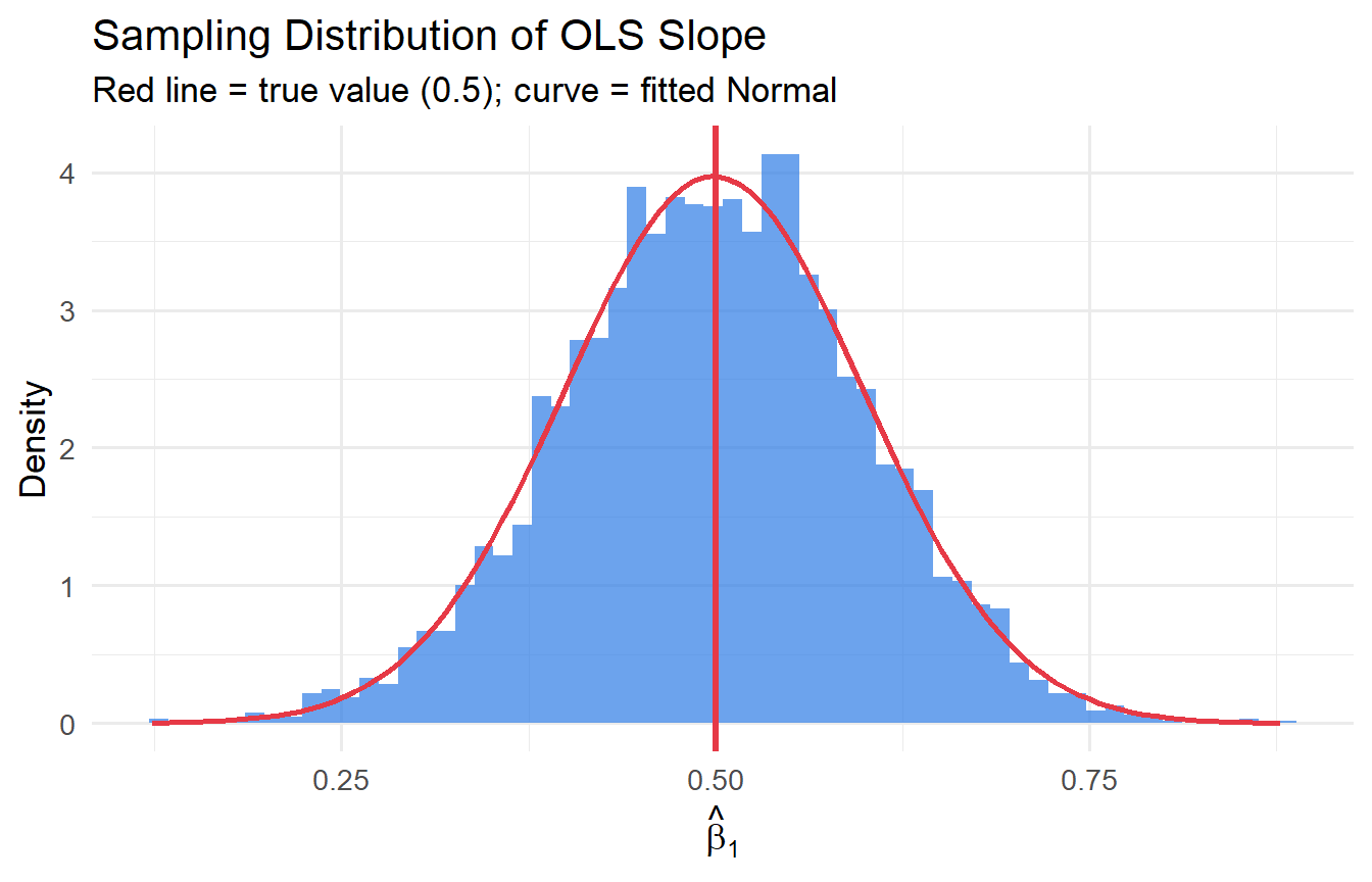
Across 5,000 simulations, $\hat{\beta}_1$ averages approximately 0.5 — confirming **unbiasedness**. We can also verify against the formula: $\text{Var}(\hat{\beta}_1) = \sigma^2 / SST_x = 4 / (n \cdot \text{Var}(x))$.
```{r}
#| label: variance-check
# Theoretical SE: sigma^2 / E[SST_x]
# E[SST_x] ≈ n * Var(x) = 50 * (10^2/12) ≈ 416.7
theoretical_var <- 4 / (50 * 100/12)
cat("Theoretical SD of slope:", round(sqrt(theoretical_var), 4), "\n")
cat("Simulation SD of slope: ", round(sd(results$slope), 4), "\n")
```
### Distribution of $\hat{\beta}_1$
```{r}
#| label: fig-sampling-dist
#| fig-cap: "Sampling distribution of OLS slope across 5,000 simulations."
ggplot(results, aes(slope)) +
  geom_histogram(aes(y = after_stat(density)), bins = 60,
                 fill = "#2c7be5", alpha = 0.7) +
  geom_vline(xintercept = 0.5, colour = "#e63946", linewidth = 1.2) +
  stat_function(fun = dnorm,
                args = list(mean = mean(results$slope), sd = sd(results$slope)),
                colour = "#e63946", linewidth = 1) +
  labs(x = expression(hat(beta)[1]), y = "Density",
       title = "Sampling Distribution of OLS Slope",
       subtitle = "Red line = true value (0.5); curve = fitted Normal")
```
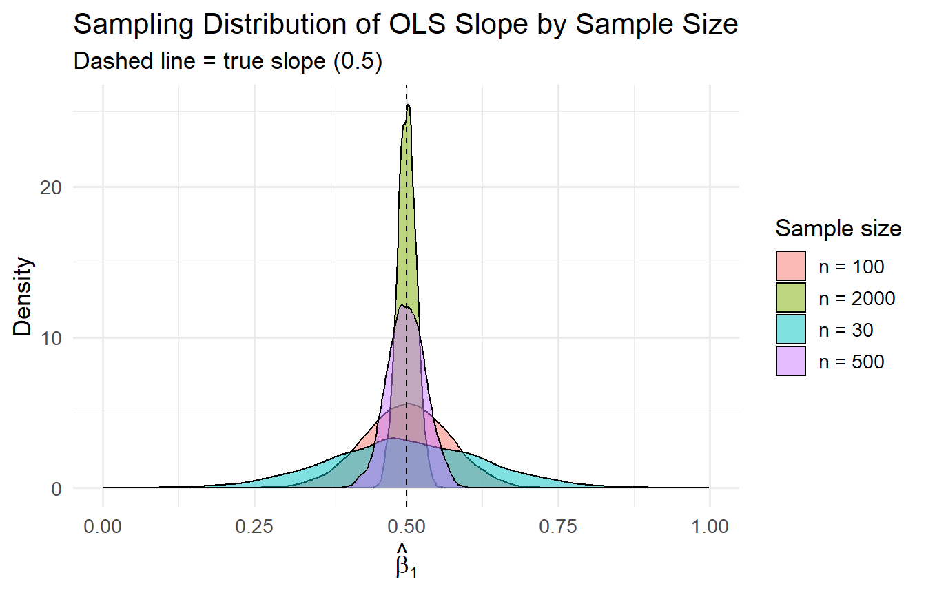
### Effect of Sample Size
```{r}
#| label: fig-sample-size
#| fig-cap: "OLS becomes more precise as n grows — consistent with Var(β̂₁) = σ²/SSTₓ."
map_dfr(c(30, 100, 500, 2000), function(n) {
  slopes <- replicate(n_sims, run_ols(n)[2])
  tibble(n = n, slope = slopes)
}) |>
  mutate(n_label = paste("n =", n)) |>
  ggplot(aes(slope, fill = n_label)) +
  geom_density(alpha = 0.5) +
  geom_vline(xintercept = 0.5, linetype = "dashed") +
  labs(x = expression(hat(beta)[1]), y = "Density", fill = "Sample size",
       title = "Sampling Distribution of OLS Slope by Sample Size",
       subtitle = "Dashed line = true slope (0.5)")
```
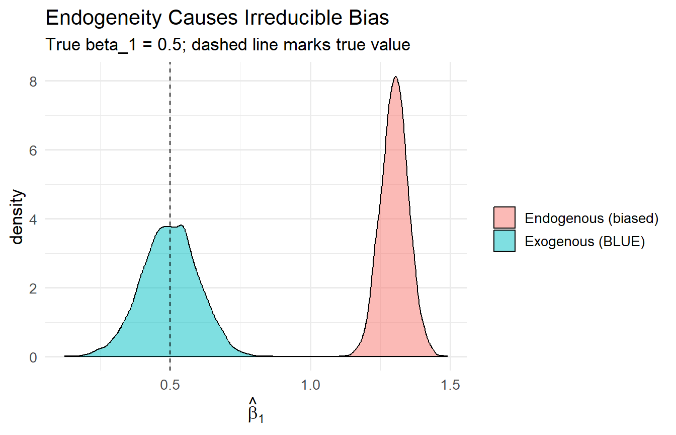
### What Happens When SLR.4 Fails? (Endogeneity)
```{r}
#| label: fig-endogeneity
#| fig-cap: "OLS is biased when the error is correlated with x. More data does not fix this."
run_biased_ols <- function(n, beta_1 = 0.5) {
  x <- runif(n, 0, 10)
  u <- 0.8 * x + rnorm(n, 0, 1)   # u correlated with x
  y <- 2 + beta_1 * x + u
  coef(lm(y ~ x))[2]
}

slopes_biased   <- replicate(n_sims, run_biased_ols(50))
slopes_unbiased <- results$slope

tibble(
  estimate = c(slopes_biased, slopes_unbiased),
  type     = rep(c("Endogenous (biased)", "Exogenous (BLUE)"), each = n_sims)
) |>
  ggplot(aes(estimate, fill = type)) +
  geom_density(alpha = 0.5) +
  geom_vline(xintercept = 0.5, linetype = "dashed") +
  labs(x = expression(hat(beta)[1]), fill = "",
       title = "Endogeneity Causes Irreducible Bias",
       subtitle = "True beta_1 = 0.5; dashed line marks true value")
```
When $\text{Cov}(x, u) \neq 0$, OLS is systematically biased — larger $n$ tightens the distribution around the *wrong* value. This motivates the search for exogenous variation (instruments, natural experiments, randomised assignment) in causal inference.
---
## Tutorials
**Tutorial 4.1**
Show algebraically that $\text{Var}(\hat{\beta}_1 \mid \mathbf{x}) = \sigma^2 / SST_x$ starting from $\hat{\beta}_1 = \beta_1 + \sum w_i u_i$ where $w_i = (x_i - \bar{x}) / SST_x$.
::: {.callout-tip collapse="true"}
## Solution
Let $S_{xx} = SST_x$ and $w_i = (x_i - \bar{x})/S_{xx}$.
$$\text{Var}(\hat{\beta}_1 \mid \mathbf{x}) = \text{Var}\!\left(\sum w_i u_i \mid \mathbf{x}\right) = \sum w_i^2 \text{Var}(u_i \mid \mathbf{x}) \stackrel{\text{SLR.5}}{=} \sigma^2 \sum w_i^2$$
$$\sum w_i^2 = \sum \frac{(x_i - \bar{x})^2}{S_{xx}^2} = \frac{S_{xx}}{S_{xx}^2} = \frac{1}{S_{xx}}$$
Therefore $\text{Var}(\hat{\beta}_1 \mid \mathbf{x}) = \sigma^2 / S_{xx} = \sigma^2 / SST_x$. $\blacksquare$
:::
**Tutorial 4.2**
Using the `wage1` dataset from `wooldridge`, regress `lwage` (log wage) on `educ` and `exper`. Separately regress `exper` on `educ`. Use the OVB formula to predict what the slope on `educ` would be if you omit `exper`. Verify by running the short regression.
::: {.callout-tip collapse="true"}
## Solution
```{r}
#| label: ex4-2
data(wage1, package = "wooldridge")

long_fit <- lm(lwage ~ educ + exper, data = wage1)
aux_fit  <- lm(exper ~ educ, data = wage1)
short_fit <- lm(lwage ~ educ, data = wage1)

beta2  <- coef(long_fit)["exper"]
delta1 <- coef(aux_fit)["educ"]

cat("Long model  beta_educ =", round(coef(long_fit)["educ"], 4), "\n")
cat("OVB prediction =", round(beta2 * delta1, 4), "\n")
cat("Short model beta_educ =", round(coef(short_fit)["educ"], 4), "\n")
cat("Matches long + OVB?   =",
    round(coef(long_fit)["educ"] + beta2 * delta1, 4), "\n")
```
The short-model coefficient on `educ` equals the long-model coefficient plus the predicted OVB — exactly. Note that `delta1 < 0` (more educated workers have fewer years of experience, given age), so omitting experience *understates* the return to education when $\beta_2 > 0$.
:::
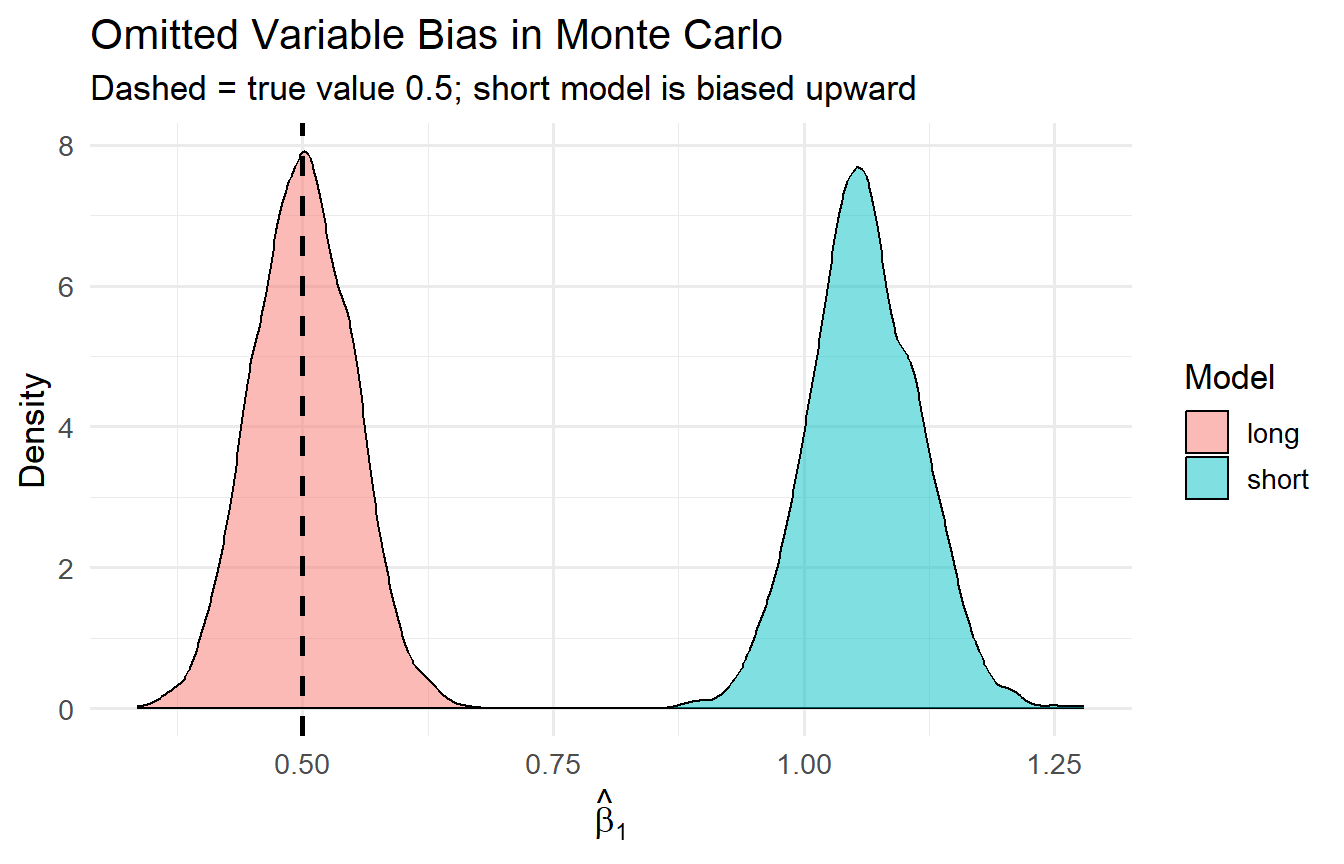
**Tutorial 4.3**
Adapt the Monte Carlo simulation to demonstrate OVB. Generate data from: $y_i = 1 + 0.5x_{1i} + 0.8x_{2i} + u_i$ where $x_{2i} = 0.7x_{1i} + v_i$. Run 2,000 simulations. In each, estimate both the long model and the short model. Plot the sampling distributions of $\tilde{\beta}_1$ (short) and $\hat{\beta}_1$ (long) and compare to the true value 0.5.
::: {.callout-tip collapse="true"}
## Solution
```{r}
#| label: ex4-3
#| fig-cap: "OVB: the short-model slope is centred above the true value; the long model recovers it."
set.seed(2024)
n_sims2 <- 2000

simulate_ovb <- function(n = 200) {
  x1 <- rnorm(n)
  x2 <- 0.7 * x1 + rnorm(n, sd = sqrt(1 - 0.7^2))
  u  <- rnorm(n, sd = 0.5)
  y  <- 1 + 0.5 * x1 + 0.8 * x2 + u

  long_b1  <- coef(lm(y ~ x1 + x2))[2]
  short_b1 <- coef(lm(y ~ x1))[2]
  tibble(long = long_b1, short = short_b1)
}

sim_results <- map_dfr(1:n_sims2, ~simulate_ovb())

sim_results |>
  pivot_longer(everything(), names_to = "model", values_to = "slope") |>
  ggplot(aes(slope, fill = model)) +
  geom_density(alpha = 0.5) +
  geom_vline(xintercept = 0.5, linetype = "dashed", linewidth = 1) +
  labs(x = expression(hat(beta)[1]), y = "Density", fill = "Model",
       title = "Omitted Variable Bias in Monte Carlo",
       subtitle = "Dashed = true value 0.5; short model is biased upward")
```
The long-model estimator is centred at 0.5. The short-model estimator is centred at $0.5 + 0.8 \times 0.7 = 1.06$ — the OVB formula in action.
:::