# FDL(2) model: fertility on tax exemption with 2 lags
fit_fdl2 <- dynlm(gfr ~ pe + L(pe, 1) + L(pe, 2) + ww2 + pill,
                  data = ts(fertil3))

tidy(fit_fdl2)Chapter 11: Dynamic Models and Distributed Lags
Modelling time dynamics: FDL, ARDL, and long-run effects
NoteLearning Objectives
By the end of this chapter you will be able to:
- Distinguish between static and dynamic regression models
- Specify and interpret Finite Distributed Lag (FDL) models
- Compute impact, interim, and long-run multipliers
- Specify and estimate Autoregressive Distributed Lag (ARDL) models using
dynlm - Explain why including lagged dependent variables affects serial correlation tests
- Interpret short-run and long-run effects in an ARDL model
1 Stationarity of AR Processes
Before specifying dynamic models, we need the concept of stationarity for AR processes, which determines whether OLS on time-series data has standard asymptotic properties.
1.1 Stationary AR(1)
An AR(1) process \(y_t = \rho y_{t-1} + e_t\) with \(e_t \sim \text{i.i.d.}(0, \sigma_e^2)\) is covariance-stationary if and only if \(|\rho| < 1\).
Mean. In stationarity, \(E[y_t] = E[y_{t-1}]\). Taking expectations: \(\mu = \rho\mu\) implies \(\mu(1-\rho) = 0\), so \(\mu = 0\) (or incorporate a constant: if \(y_t = \alpha + \rho y_{t-1} + e_t\) then \(\mu = \alpha/(1-\rho)\)).
Variance. \(\text{Var}(y_t) = \rho^2 \text{Var}(y_{t-1}) + \sigma_e^2\). In stationarity, \(\text{Var}(y_t) = \text{Var}(y_{t-1}) = \gamma_0\):
\[\gamma_0 = \rho^2 \gamma_0 + \sigma_e^2 \implies \gamma_0 = \frac{\sigma_e^2}{1 - \rho^2}\]
This is finite if and only if \(|\rho| < 1\).
Autocovariance. \(\gamma(h) = \text{Cov}(y_t, y_{t-h}) = \rho^h \gamma_0\), so the autocorrelation function is:
\[\text{Corr}(y_t, y_{t-h}) = \rho^h\]
The ACF decays geometrically — slowly for \(\rho\) near 1, quickly for \(\rho\) near 0. For \(\rho = 1\) (a random walk), \(\gamma_0 = \infty\) and the ACF does not decay (the process is non-stationary).
1.2 AR(p) and the Stationarity Condition
A general AR(\(p\)) process: \(y_t = \rho_1 y_{t-1} + \cdots + \rho_p y_{t-p} + e_t\) is stationary if and only if all roots of the characteristic polynomial \(1 - \rho_1 z - \cdots - \rho_p z^p = 0\) lie outside the unit circle in the complex plane. For AR(1), this reduces to \(|\rho| < 1\).
2 Static vs. Dynamic Models
All the regression models in Chapters 3–10 were static: the effect of \(x_t\) on \(y_t\) was assumed to occur instantly and completely within period \(t\).
In time-series economics, this is often unrealistic. Investment decisions, price adjustments, and behavioural responses all take time. We need dynamic models that capture these lags.
| Model type | Specification | Key feature |
|---|---|---|
| Static | \(y_t = \beta_0 + \beta_1 x_t + u_t\) | Instantaneous adjustment |
| FDL(\(q\)) | \(y_t = \alpha_0 + \delta_0 x_t + \delta_1 x_{t-1} + \cdots + \delta_q x_{t-q} + u_t\) | Lagged effects of \(x\) |
| ARDL(\(p,q\)) | \(y_t = \alpha_0 + \sum_{j=1}^p \rho_j y_{t-j} + \sum_{j=0}^q \delta_j x_{t-j} + u_t\) | Lagged \(y\) and \(x\) |
3 Finite Distributed Lag (FDL) Models
A Finite Distributed Lag model of order \(q\) allows \(x\) to affect \(y\) over \(q + 1\) periods:
\[ y_t = \alpha_0 + \delta_0 x_t + \delta_1 x_{t-1} + \delta_2 x_{t-2} + \cdots + \delta_q x_{t-q} + u_t \]
3.1 Multipliers
| Multiplier | Definition | Interpretation |
|---|---|---|
| Impact multiplier | \(\delta_0\) | Immediate effect of \(\Delta x_t\) on \(y_t\) |
| \(s\)-period multiplier | \(\delta_s\) | Effect \(s\) periods after the change |
| Interim multiplier (period \(m\)) | \(\sum_{s=0}^m \delta_s\) | Cumulative effect after \(m+1\) periods |
| Long-run multiplier (LRM) | \(\sum_{s=0}^q \delta_s\) | Total cumulative effect of a permanent \(\Delta x\) |
3.2 Example: Fertility and Tax Exemptions
How does a personal tax exemption for children affect the general fertility rate? Economic theory predicts a positive long-run effect (lower cost of children), but the response may be delayed.
b <- coef(fit_fdl2)

impact    <- b["pe"]
interimL1 <- b["pe"] + b["L(pe, 1)"]
lrm       <- b["pe"] + b["L(pe, 1)"] + b["L(pe, 2)"]

cat("Impact multiplier (period 0):", round(impact, 3), "\n")
Impact multiplier (period 0): 0.073 cat("Interim multiplier (period 1):", round(interimL1, 3), "\n")Interim multiplier (period 1): 0.067 cat("Long-run multiplier (LRM): ", round(lrm, 3), "\n")Long-run multiplier (LRM): 0.101 tibble(
period = 0:2,
delta = c(b["pe"], b["L(pe, 1)"], b["L(pe, 2)"]),
cumulative = cumsum(c(b["pe"], b["L(pe, 1)"], b["L(pe, 2)"]))
) |>
ggplot(aes(period, delta)) +
geom_col(fill = "#2c7be5", width = 0.5) +
geom_line(aes(y = cumulative), colour = "#e63946", linewidth = 1.2) +
geom_point(aes(y = cumulative), colour = "#e63946", size = 3) +
scale_x_continuous(breaks = 0:2) +
labs(x = "Lag (years)", y = "Effect on GFR",
title = "Distributed Lag Profile: Tax Exemption → Fertility",
subtitle = "Bars = lag coefficients; red line = cumulative (interim multiplier)")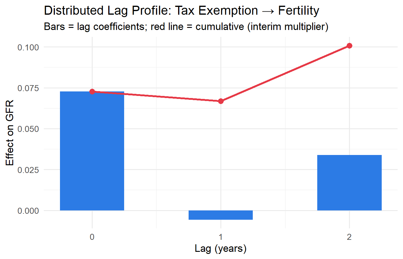
TipUsing
dynlm
The dynlm package lets you write lag operators directly in the formula: - L(x) = \(x_{t-1}\) (one lag) - L(x, 2) = \(x_{t-2}\) (two lags) - d(x) = \(\Delta x_t = x_t - x_{t-1}\) (first difference) - L(d(x)) = \(\Delta x_{t-1}\)
This avoids manually creating lag columns and handles the time-series structure automatically.
4 Autoregressive Distributed Lag (ARDL) Models
An ARDL(\(p, q\)) model includes lags of both \(y\) and \(x\):
\[ y_t = \alpha_0 + \rho_1 y_{t-1} + \cdots + \rho_p y_{t-p} + \delta_0 x_t + \cdots + \delta_q x_{t-q} + u_t \]
The lagged dependent variable \(y_{t-1}\) captures persistence — the tendency for \(y\) to remain near its past level.
4.1 Why Include Lagged \(y\)?
- Economic theory: partial adjustment, habit formation, adaptive expectations
- Serial correlation fix: including \(y_{t-1}\) often eliminates AR(1) errors if the static model was misspecified (check with BG test — not DW, which is invalid here)
- Parsimonious dynamics: \(y_{t-1}\) absorbs the effect of many distant lags of \(x\)
4.2 Long-Run Multiplier in ARDL
For an ARDL(1,1) model: \[ y_t = \alpha_0 + \rho y_{t-1} + \delta_0 x_t + \delta_1 x_{t-1} + u_t \]
In the long run, \(y_t = y_{t-1} = y^*\) and \(x_t = x_{t-1} = x^*\). Solving:
\[ \text{LRM} = \frac{\delta_0 + \delta_1}{1 - \rho} \]
The denominator \(1 - \rho\) amplifies the long-run effect — the more persistent the process, the larger the long-run multiplier.
4.3 Example: Housing Investment and Interest Rates
hseinv_ts <- ts(hseinv, start = 1947)

# Static model: log investment per capita on log price + time trend
fit_static <- dynlm(log(invpc) ~ log(price) + t, data = hseinv_ts)

# ARDL(1,1): add lagged dependent variable and one lag of log(price)
fit_ardl11 <- dynlm(log(invpc) ~ L(log(invpc)) + log(price) + L(log(price)) + t,
                    data = hseinv_ts)

modelsummary(
  list("Static" = fit_static, "ARDL(1,1)" = fit_ardl11),
  stars   = TRUE,
  gof_map = c("nobs", "r.squared", "adj.r.squared"),
  title   = "Housing Investment: Static vs. ARDL(1,1)"
)| Static | ARDL(1,1) | |
|---|---|---|
| + p < 0.1, * p < 0.05, ** p < 0.01, *** p < 0.001 | ||
| (Intercept) | -0.913*** | -0.795*** |
| (0.136) | (0.151) | |
| log(price) | -0.381 | 2.452* |
| (0.679) | (0.933) | |
| t | 0.010** | 0.011*** |
| (0.004) | (0.003) | |
| L(log(invpc)) | 0.344** | |
| (0.126) | ||
| L(log(price)) | -3.701*** | |
| (0.929) | ||
| Num.Obs. | 42 | 41 |
| R2 | 0.341 | 0.639 |
| R2 Adj. | 0.307 | 0.599 |
b_ardl <- coef(fit_ardl11)
rho_hat <- b_ardl["L(log(invpc))"]
delta0  <- b_ardl["log(price)"]
delta1  <- b_ardl["L(log(price))"]

lrm_ardl <- (delta0 + delta1) / (1 - rho_hat)
cat("Short-run effect of log(price):", round(delta0, 4), "\n")
Short-run effect of log(price): 2.452 cat("Estimated rho (persistence): ", round(rho_hat, 4), "\n")Estimated rho (persistence): 0.3445 cat("Long-run multiplier (LRM): ", round(lrm_ardl, 4), "\n")Long-run multiplier (LRM): -1.907 # BG test for serial correlation (DW is invalid with lagged y)
bgtest(fit_ardl11, order = 2)
    Breusch-Godfrey test for serial correlation of order up to 2

data:  fit_ardl11
LM test = 8.7, df = 2, p-value = 0.01
The BG test checks whether adding \(y_{t-1}\) has resolved the serial correlation problem. If not significant, the ARDL specification adequately captures the dynamics.
4.4 AR-Error Models vs. ARDL: A Key Distinction
In Chapter 10, we modelled serial correlation in the error term as AR(1): \(u_t = \rho u_{t-1} + e_t\). This is different from including a lagged dependent variable.
When the true DGP is ARDL(1,0): \(y_t = \alpha + \phi y_{t-1} + \delta x_t + e_t\), but we estimate the static model \(y_t = \alpha + \delta x_t + u_t\), the error satisfies \(u_t = \phi u_{t-1} + e_t - \phi\delta(x_t - x_{t-1}) + \ldots\). The AR-error structure imposes a geometric lag structure on the FDL: the coefficients on \(x_{t-1}, x_{t-2}, \ldots\) must satisfy \(\delta_s = \phi^s \delta_0\) — a very restrictive pattern. The ARDL is more flexible: it allows the distributed lag profile to take any shape.
In practice: - If serial correlation arises from model misspecification (missing dynamics), use an ARDL — it fixes the problem and restores valid inference. - If serial correlation arises from data persistence in the error (e.g., measurement error is autocorrelated), then HAC SEs or FGLS are appropriate.
4.5 Central Bank Reaction Function: An ARDL Example
Central banks set interest rates responding to inflation and the output gap, but with inertia — rates do not jump immediately to their target. The standard Taylor rule with interest rate smoothing:
\[i_t = \alpha(1-\rho) + \rho i_{t-1} + \beta_\pi(1-\rho)\pi_t + \beta_y(1-\rho)g_t + e_t\]
where \(\rho\) captures smoothing (inertia). This is an ARDL(1,2).
# Use intdef as a proxy: i3 ~ lagged i3 + inflation
data("intdef", package = "wooldridge")
intdef_ts <- ts(intdef, start = 1948)

fit_taylor <- dynlm(i3 ~ L(i3) + inf + def, data = intdef_ts)
tidy(fit_taylor)
b_tr <- coef(fit_taylor)
rho_tr <- b_tr["L(i3)"]
cat("Smoothing parameter rho: ", round(rho_tr, 4), "\n")Smoothing parameter rho: 0.7184 cat("Long-run effect of inflation: ", round(b_tr["inf"] / (1 - rho_tr), 4), "\n")Long-run effect of inflation: 1.024 cat("Long-run effect of deficit: ", round(b_tr["def"] / (1 - rho_tr), 4), "\n")Long-run effect of deficit: -0.2055 The long-run multiplier on inflation is \(\hat{\beta}_{inf}/(1-\hat{\rho})\) — amplified by the persistence of interest rates.
4.6 Partial Adjustment Interpretation
The ARDL(1,0) model has a natural interpretation as a partial adjustment model:
\[ y_t - y_{t-1} = \lambda(y_t^* - y_{t-1}) \quad \text{where} \quad y_t^* = \alpha + \beta x_t \]
If \(y\) adjusts only partially toward its equilibrium \(y_t^*\) each period, then:
\[ y_t = \lambda \alpha + (1 - \lambda) y_{t-1} + \lambda \beta x_t \]
This is an ARDL(1,0) with \(\rho = 1 - \lambda\) (speed of adjustment) and \(\delta_0 = \lambda \beta\) (short-run response). The long-run effect is \(\beta = \delta_0 / (1 - \rho)\).
5 Static vs. Dynamic: A Comparison
# Simulate impulse responses
shock <- c(1, rep(0, 9))  # one-time shock at t=1

# FDL(3): direct lag effects
fdl_coeffs <- c(0.4, 0.3, 0.2, 0.1)  # illustrative
fdl_response <- convolve(shock, rev(fdl_coeffs), type = "open")[1:10]

# ARDL(1,0): geometric decay
rho_ex  <- 0.7
delta_ex <- 0.5
ardl_response <- numeric(10)
ardl_response[1] <- delta_ex
for (t in 2:10) ardl_response[t] <- rho_ex * ardl_response[t-1]

tibble(
  t       = 1:10,
  FDL     = fdl_response,
  ARDL    = ardl_response
) |>
  pivot_longer(-t, names_to = "model", values_to = "response") |>
  ggplot(aes(t, response, colour = model, group = model)) +
  geom_line(linewidth = 1.2) +
  geom_point(size = 2.5) +
  geom_hline(yintercept = 0, linetype = "dashed") +
  scale_x_continuous(breaks = 1:10) +
  labs(x = "Periods after shock", y = "Response of y",
       colour = "Model",
       title = "Impulse Response Functions",
       subtitle = "FDL = finite lag structure; ARDL = geometric decay")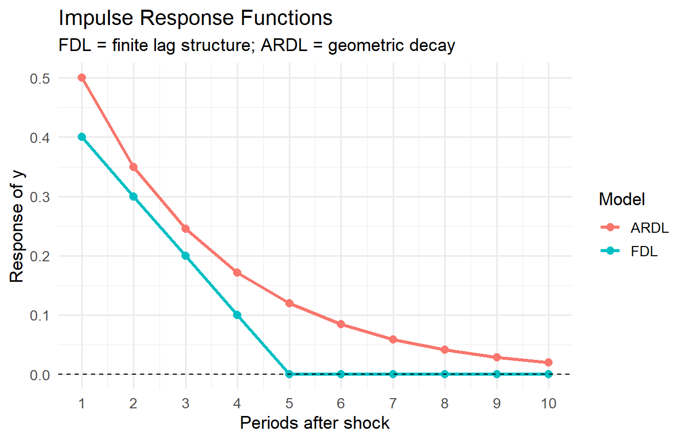
6 Tutorials
Tutorial 11.1 Using wooldridge::fertil3, estimate an FDL(2) model of the general fertility rate (gfr) on the personal tax exemption (pe) — no controls. Compute and interpret:
- The impact multiplier
- The 2-period interim multiplier
- The long-run multiplier
Is the long-run effect positive, as economic theory predicts?
TipSolution
fit_fdl2_simple <- dynlm(gfr ~ pe + L(pe, 1) + L(pe, 2), data = ts(fertil3))
tidy(fit_fdl2_simple)
b2 <- coef(fit_fdl2_simple)
cat("Impact multiplier: ", round(b2["pe"], 3), "\n")Impact multiplier: -0.016 cat("2-period interim mult.: ", round(sum(b2[c("pe","L(pe, 1)","L(pe, 2)")][1:2]), 3), "\n")2-period interim mult.: -0.037 cat("Long-run multiplier: ", round(sum(b2[c("pe","L(pe, 1)","L(pe, 2)")]), 3), "\n")Long-run multiplier: 0.017 The long-run multiplier should be positive: a permanent $1 increase in the tax exemption per child eventually raises the fertility rate. The impact multiplier may be smaller (or even negative) as people adjust expectations — the full effect accumulates over two years.
Tutorial 11.2 Add a lagged dependent variable to the Phillips curve model (inf ~ unem, wooldridge::phillips) to create an ARDL(1,0). Compare:
- Static OLS vs. ARDL(1,0): how do the estimated effects of unemployment on inflation change?
- Does the ARDL specification resolve serial correlation? Apply the BG test (order 1).
- Compute the long-run effect of unemployment on inflation from the ARDL model.
TipSolution
fit_static_ph <- dynlm(inf ~ unem, data = ts(phillips, start = 1948))
fit_ardl_ph   <- dynlm(inf ~ L(inf) + unem, data = ts(phillips, start = 1948))

modelsummary(
  list("Static" = fit_static_ph, "ARDL(1,0)" = fit_ardl_ph),
  stars = TRUE, gof_map = c("nobs", "r.squared"),
  title = "Phillips Curve: Static vs. ARDL(1,0)"
)| Static | ARDL(1,0) | |
|---|---|---|
| + p < 0.1, * p < 0.05, ** p < 0.01, *** p < 0.001 | ||
| (Intercept) | 1.054 | 2.210+ |
| (1.548) | (1.210) | |
| unem | 0.502+ | -0.224 |
| (0.266) | (0.239) | |
| L(inf) | 0.733*** | |
| (0.117) | ||
| Num.Obs. | 56 | 55 |
| R2 | 0.062 | 0.477 |
# BG test on ARDL
bgtest(fit_ardl_ph, order = 1)
    Breusch-Godfrey test for serial correlation of order up to 1

data:  fit_ardl_ph
LM test = 2.2, df = 1, p-value = 0.1
# Long-run multiplier
b_ph <- coef(fit_ardl_ph)
lrm_ph <- b_ph["unem"] / (1 - b_ph["L(inf)"])
cat("LRM (unemployment -> inflation):", round(lrm_ph, 4), "\n")LRM (unemployment -> inflation): -0.8391 The static model likely has significant serial correlation (BG test). The ARDL model should reduce or eliminate it. The short-run and long-run effects of unemployment on inflation will differ — the long-run multiplier amplifies the short-run coefficient by \(1/(1-\hat{\rho})\).
Tutorial 11.3 Explain the difference between the impact multiplier and the long-run multiplier in an FDL model. Under what conditions is the long-run multiplier much larger than the impact multiplier? Provide an economic example.
TipSolution
The impact multiplier (\(\delta_0\)) measures the immediate, within-period response of \(y\) to a unit change in \(x\). The long-run multiplier (\(\sum_{s=0}^q \delta_s\)) measures the total cumulative response after all lag effects have worked through.
The LRM is much larger than the impact multiplier when: 1. The lag coefficients \(\delta_1, \ldots, \delta_q\) are large and positive — the effects of \(x\) accumulate over many periods 2. In ARDL models, when \(\rho\) (persistence) is close to 1, the denominator \((1-\rho)\) becomes small, amplifying the LRM
Economic example: Consider the effect of a sustained monetary policy change on inflation. In the short run, monetary policy operates with a lag — the impact multiplier might be near zero. Over 12–24 months, however, prices adjust and the full disinflationary effect materialises. The long-run multiplier captures the total reduction in inflation from a permanent 1 percentage point change in the interest rate, which can be several times larger than the impact effect.