---
title: "Chapter 9: Heteroskedasticity"
subtitle: "Detection, consequences, and robust inference"
---
```{r}
#| label: setup
#| include: false
library(tidyverse)
library(broom)
library(modelsummary)
library(lmtest)
library(sandwich)
library(estimatr)
library(wooldridge)
theme_set(theme_minimal(base_size = 13))
options(digits = 4, scipen = 999)
data("hprice1", package = "wooldridge")
data("wage1", package = "wooldridge")
```
::: {.callout-note}
## Learning Objectives
By the end of this chapter you will be able to:
- Define heteroskedasticity and explain why it matters for inference
- Detect heteroskedasticity using graphical methods, the Breusch-Pagan test, and the White test
- Explain why OLS remains unbiased but standard errors become invalid under heteroskedasticity
- Compute and interpret heteroskedasticity-robust standard errors using `sandwich` and `estimatr`
- Apply Weighted Least Squares (WLS) as an efficient estimator when the error variance structure is known
:::
---
## What Is Heteroskedasticity?
**Homoskedasticity** (SLR.5) requires $\text{Var}(u \mid x) = \sigma^2$ — constant variance across all values of $x$.
**Heteroskedasticity** occurs when this fails:
$$
\text{Var}(u_i \mid x_i) = \sigma_i^2 \quad \text{(varies across observations)}
$$
This is common in cross-sectional data. For example:
- Housing prices: larger houses have more variable prices
- Wages: variation in wages tends to be higher among high-education workers
- Firm-level data: large firms have more volatile outcomes than small firms
### Consequences of Heteroskedasticity
| Property | Under Homoskedasticity | Under Heteroskedasticity |
|---|---|---|
| OLS unbiased? | Yes (SLR.1–4 sufficient) | **Yes** — unbiasedness unchanged |
| OLS consistent? | Yes | **Yes** — consistency unchanged |
| OLS BLUE? | Yes (Gauss-Markov) | **No** — WLS is more efficient |
| Standard SE formula valid? | Yes | **No** — SEs are biased |
| t and F tests valid? | Yes | **No** — tests are wrong |
The key point: **heteroskedasticity does not bias the coefficients, but it invalidates the standard errors** — and therefore all hypothesis tests and confidence intervals.
---
## Visualising Heteroskedasticity
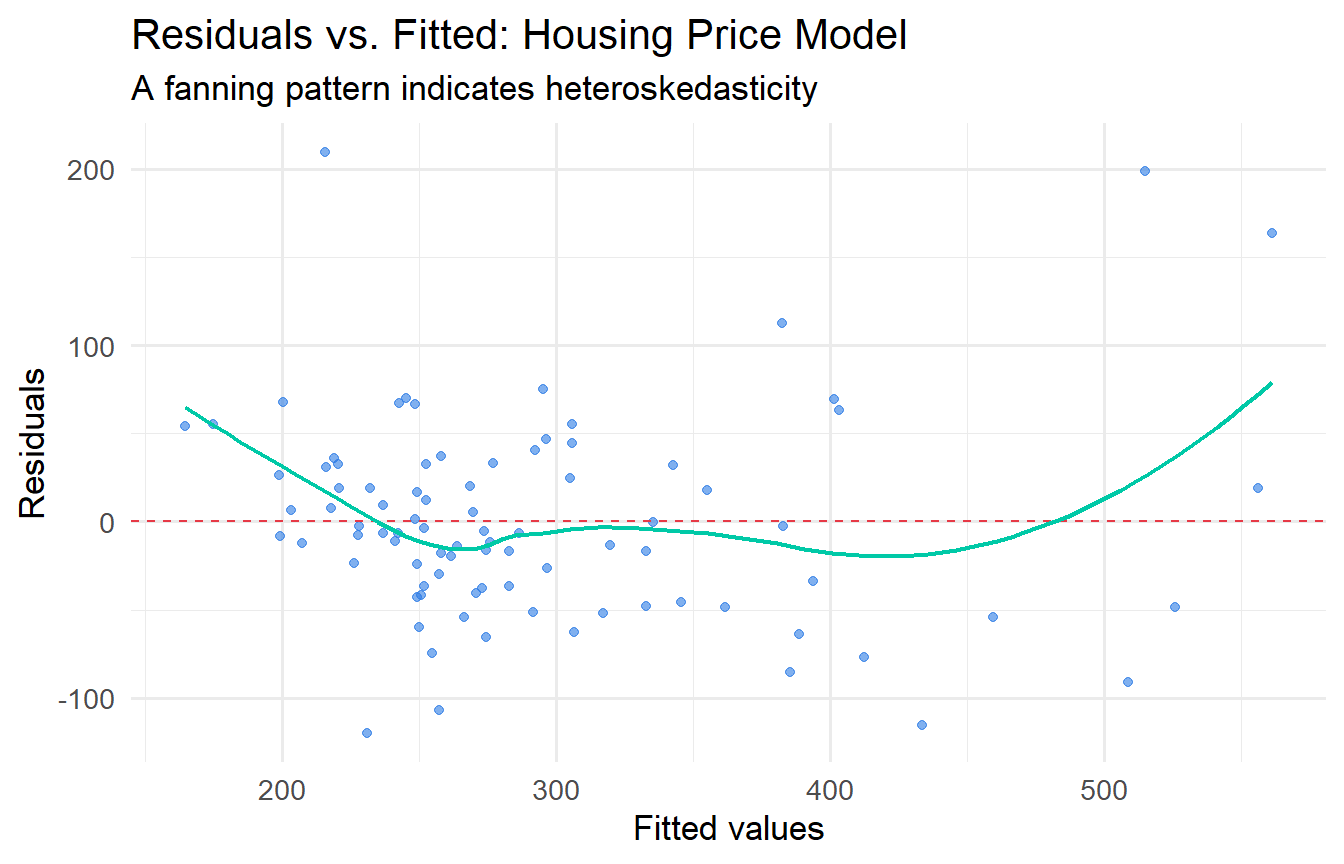
The most informative diagnostic is a plot of residuals against fitted values (or against $x$).
```{r}
#| label: fig-resid-plot
#| fig-cap: "Residual plot for the housing price model. Fan shape suggests heteroskedasticity."
fit_hprice <- lm(price ~ sqrft + bdrms + lotsize, data = hprice1)

augment(fit_hprice) |>
  ggplot(aes(.fitted, .resid)) +
  geom_point(alpha = 0.6, colour = "#2c7be5") +
  geom_hline(yintercept = 0, linetype = "dashed", colour = "#e63946") +
  geom_smooth(method = "loess", se = FALSE, colour = "#00c9a7", linewidth = 0.8) +
  labs(x = "Fitted values", y = "Residuals",
       title = "Residuals vs. Fitted: Housing Price Model",
       subtitle = "A fanning pattern indicates heteroskedasticity")
```
```{r}
#| label: fig-scale-location
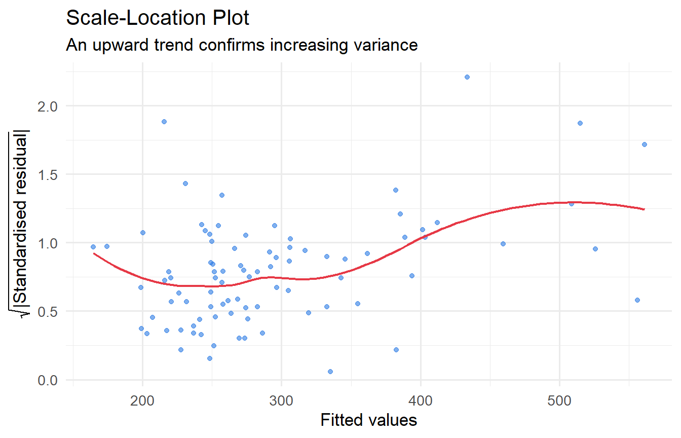
#| fig-cap: "Scale-location plot: sqrt(|residuals|) against fitted values."
augment(fit_hprice) |>
  mutate(sqrt_abs_resid = sqrt(abs(.std.resid))) |>
  ggplot(aes(.fitted, sqrt_abs_resid)) +
  geom_point(alpha = 0.6, colour = "#2c7be5") +
  geom_smooth(method = "loess", se = FALSE, colour = "#e63946", linewidth = 0.8) +
  labs(x = "Fitted values", y = expression(sqrt("|Standardised residual|")),
       title = "Scale-Location Plot",
       subtitle = "An upward trend confirms increasing variance")
```
The clear upward trend confirms that variance increases with house price — a classic case of heteroskedasticity in housing data.
---
## Formal Tests for Heteroskedasticity
### Breusch-Pagan Test
The **Breusch-Pagan (BP) test** is a formal Lagrange Multiplier test of the null hypothesis that errors are homoskedastic.
**Setup.** Suppose the true error variance is a linear function of auxiliary variables $\mathbf{z}_i = (z_{i1}, \ldots, z_{iq})'$:
$$H_0: \sigma_i^2 = \sigma^2 \quad (\text{constant for all } i)$$
$$H_1: \sigma_i^2 = \sigma^2 + \alpha_1 z_{i1} + \cdots + \alpha_q z_{iq}$$
Often $\mathbf{z}_i = \mathbf{x}_i$ (the original regressors), but the test is valid for any choice.
**Procedure:**
1. Estimate the original model and obtain $\hat{u}_i^2$
2. Regress $\hat{u}_i^2$ on $z_{i1}, \ldots, z_{iq}$ and record $R^2_{\hat{u}^2}$
3. The test statistic $LM = nR^2_{\hat{u}^2} \xrightarrow{d} \chi^2(q)$ under $H_0$
A significant result rejects the null of homoskedasticity.
```{r}
#| label: bp-test
bptest(fit_hprice)
```
```{r}
#| label: bp-test-log
# Log specification often reduces heteroskedasticity
fit_log <- lm(log(price) ~ log(sqrft) + bdrms + log(lotsize), data = hprice1)
bptest(fit_log)
```
The BP test strongly rejects homoskedasticity for the level model. The log-log specification reduces (but does not eliminate) heteroskedasticity — log transformations often stabilise variance.
### White Test
The **White (1980) test** is more general than the BP test. The full White test regresses $\hat{u}_i^2$ on all regressors, their squares, and all cross-products:
$$\hat{u}_i^2 = \alpha_0 + \sum_j \alpha_j x_{ij} + \sum_j \alpha_{jj} x_{ij}^2 + \sum_{j < \ell} \alpha_{j\ell} x_{ij} x_{i\ell} + v_i$$
With $k$ regressors, there are $k + k + \binom{k}{2} = k(k+3)/2$ auxiliary regressors, so the $\chi^2$ degrees of freedom grow quickly.
**The special form** (using fitted values) avoids this proliferation. Note that $\hat{y}_i = \hat{\beta}_0 + \hat{\beta}_1 x_{1i} + \cdots + \hat{\beta}_k x_{ki}$ is a linear combination of the regressors, and $\hat{y}_i^2$ is a linear combination of all squares and cross-products. So regressing $\hat{u}_i^2$ on $\hat{y}_i$ and $\hat{y}_i^2$ captures a projection onto the same space as the full White test, but with only 2 auxiliary variables instead of $k(k+3)/2$.
```{r}
#| label: white-test
# White test (special form): regress u^2 on yhat and yhat^2
bptest(fit_hprice, ~ fitted(fit_hprice) + I(fitted(fit_hprice)^2))
```
The White test detects heteroskedasticity that the BP test misses when the variance depends non-linearly on the regressors.
::: {.callout-tip}
## BP vs. White
- **BP test**: tests for heteroskedasticity that is a linear function of the regressors. Easy to interpret.
- **White test**: tests for any form of heteroskedasticity, including non-linear. More general but harder to diagnose.
- Both are large-sample tests justified by asymptotic theory (Chapter 8). The p-value comes from $\chi^2$ critical values.
:::
---
## The Solution: Robust Standard Errors
### The Sandwich Estimator: Derivation
Since Chapter 8 established that OLS is consistent under weak conditions, we can keep OLS for estimation. The fix for inference is to replace the biased standard SE formula with **heteroskedasticity-robust standard errors**.
The need arises from the general variance formula derived in Chapter 8. Under heteroskedasticity, let $\Omega = \text{Var}(\mathbf{u} \mid \mathbf{X}) = \text{diag}(\sigma_1^2, \sigma_2^2, \ldots, \sigma_n^2)$ (the true error variances, each allowed to differ). Then:
$$\text{Var}(\hat{\boldsymbol{\beta}} \mid \mathbf{X}) = (\mathbf{X}'\mathbf{X})^{-1}\mathbf{X}' \boldsymbol{\Omega} \mathbf{X}(\mathbf{X}'\mathbf{X})^{-1}$$
The "filling" of the sandwich is:
$$\mathbf{X}'\boldsymbol{\Omega}\mathbf{X} = \sum_{i=1}^n \sigma_i^2 \mathbf{x}_i\mathbf{x}_i'$$
Since $\sigma_i^2$ is unknown, we replace it with $\hat{u}_i^2$ (the squared OLS residual for observation $i$). This gives the **HC0 sandwich estimator**:
$$\widehat{\text{Var}}_{\text{HC0}}(\hat{\boldsymbol{\beta}}) = (\mathbf{X}'\mathbf{X})^{-1} \left(\sum_{i=1}^n \hat{u}_i^2 \mathbf{x}_i\mathbf{x}_i'\right) (\mathbf{X}'\mathbf{X})^{-1}$$
**Why is $\hat{u}_i^2$ a valid replacement for $\sigma_i^2$?** By consistency of OLS, $\hat{u}_i \xrightarrow{p} u_i$, so $\hat{u}_i^2 \xrightarrow{p} u_i^2$ and $E[u_i^2 \mid \mathbf{x}_i] = \sigma_i^2$. The substitution is justified asymptotically by the WLLN applied to $\sum \hat{u}_i^2 \mathbf{x}_i\mathbf{x}_i' / n \xrightarrow{p} E[\sigma_i^2 \mathbf{x}_i\mathbf{x}_i']$.
**Contrast with the standard formula.** Under homoskedasticity ($\sigma_i^2 = \sigma^2$ for all $i$):
$$\mathbf{X}'\boldsymbol{\Omega}\mathbf{X} = \sigma^2 \mathbf{X}'\mathbf{X} \implies \text{Var}(\hat{\boldsymbol{\beta}}) = \sigma^2(\mathbf{X}'\mathbf{X})^{-1}$$
The standard formula is a special case of the sandwich when the diagonal of $\boldsymbol{\Omega}$ is constant. When $\sigma_i^2$ varies, the standard formula gets the "filling" wrong — typically understating the variance when high-$x$ observations have large errors.
### HC Variants
| Variant | Filling | Recommended for |
|---|---|---|
| HC0 | $\hat{u}_i^2$ | Large $n$ |
| HC1 | $\frac{n}{n-k-1}\hat{u}_i^2$ | Default in Stata (`robust`) |
| HC3 | $\frac{\hat{u}_i^2}{(1-h_{ii})^2}$ | **Best for small/moderate $n$** |
$h_{ii} = [\mathbf{P}_X]_{ii}$ is the **leverage** of observation $i$ — how much $i$ influences its own fitted value. HC3 inflates the residuals for high-leverage observations, which tend to have understated residuals (they "pull" the fit toward themselves).
### Method 1: `sandwich` + `lmtest`
```{r}
#| label: robust-se-sandwich
# Standard OLS SEs
coeftest(fit_hprice)
# HC3 robust SEs (default, recommended for small samples)
coeftest(fit_hprice, vcov = vcovHC(fit_hprice, type = "HC3"))
```
### Method 2: `estimatr::lm_robust()`
`lm_robust()` computes robust SEs directly and integrates with `modelsummary`:
```{r}
#| label: robust-se-estimatr
fit_robust <- lm_robust(price ~ sqrft + bdrms + lotsize,
                        data = hprice1, se_type = "HC3")
tidy(fit_robust)
```
### Side-by-Side Comparison
```{r}
#| label: comparison-table
#| tbl-cap: "OLS vs. Robust SEs for housing price model."
modelsummary(
  list(
    "OLS (conventional SEs)" = fit_hprice,
    "OLS (HC3 robust SEs)"   = fit_robust
  ),
  stars   = TRUE,
  gof_map = c("nobs", "r.squared"),
  title   = "Effect of Robust SEs on Housing Price Estimates"
)
```
Notice: the **coefficient estimates are identical** — only the standard errors (and thus t-statistics and p-values) change. With robust SEs, inference is valid regardless of the form of heteroskedasticity.
::: {.callout-important}
## Which HC Variant?
The `sandwich` package provides several estimators:
| Type | Formula | Recommended when |
|---|---|---|
| HC0 | $\hat{u}_i^2$ | Large $n$ |
| HC1 | $\frac{n}{n-k-1} \hat{u}_i^2$ | Default in Stata |
| HC3 | $\frac{\hat{u}_i^2}{(1 - h_{ii})^2}$ | **Best for small/moderate $n$** |
Use HC3 by default — it corrects for leverage and performs well in finite samples. Stata's `robust` option uses HC1.
:::
---
## Weighted Least Squares (WLS)
When you *know* (or can estimate) the form of the error variance, **WLS** is more efficient than OLS with robust SEs.
### Derivation: Why WLS Restores Homoskedasticity
Suppose $\text{Var}(u_i \mid \mathbf{x}_i) = \sigma^2 h_i$ where $h_i > 0$ is known. Divide the regression equation for observation $i$ by $\sqrt{h_i}$:
$$\frac{y_i}{\sqrt{h_i}} = \frac{\beta_0}{\sqrt{h_i}} + \beta_1 \frac{x_{1i}}{\sqrt{h_i}} + \cdots + \beta_k \frac{x_{ki}}{\sqrt{h_i}} + \frac{u_i}{\sqrt{h_i}}$$
Define $y_i^* = y_i/\sqrt{h_i}$, $x_{ji}^* = x_{ji}/\sqrt{h_i}$, and $u_i^* = u_i/\sqrt{h_i}$. The transformed error:
$$\text{Var}(u_i^* \mid \mathbf{x}_i) = \frac{\text{Var}(u_i \mid \mathbf{x}_i)}{h_i} = \frac{\sigma^2 h_i}{h_i} = \sigma^2$$
The transformed model $y_i^* = \beta_0 x_{0i}^* + \beta_1 x_{1i}^* + \cdots + u_i^*$ (where $x_{0i}^* = 1/\sqrt{h_i}$, not a constant) satisfies **homoskedasticity**. OLS on the transformed data is therefore BLUE by Gauss-Markov — this is WLS.
WLS minimises:
$$\sum_{i=1}^n \frac{1}{h_i} (y_i - \beta_0 - \beta_1 x_{1i} - \cdots)^2 = \sum_{i=1}^n w_i (y_i - \mathbf{x}_i'\boldsymbol{\beta})^2, \qquad w_i = 1/h_i$$
In R, this is just `lm()` with a `weights` argument:
```{r}
#| label: wls
# Suppose variance is proportional to sqrft (larger homes => more variable prices)
fit_wls <- lm(price ~ sqrft + bdrms + lotsize,
              data = hprice1,
              weights = 1 / hprice1$sqrft)

modelsummary(
  list("OLS" = fit_hprice, "WLS (1/sqrft)" = fit_wls),
  stars   = TRUE,
  gof_map = c("nobs", "r.squared"),
  title   = "OLS vs. WLS for Housing Prices"
)
```
::: {.callout-tip}
## OLS with Robust SEs vs. WLS
- **OLS + robust SEs**: Always valid for inference; does not improve efficiency. The preferred choice when the variance structure is unknown.
- **WLS**: More efficient (smaller SEs) when the variance structure is *correctly* specified. Misspecifying the weights can make things worse.
In practice, **OLS with robust SEs is the default recommendation** for cross-sectional data. WLS is useful when the variance structure is theoretically motivated (e.g., grouped data where $h_i$ is the group size).
:::
---
## Tutorials
**Tutorial 9.1**
Using `wooldridge::wage1`, regress `wage` on `educ`, `exper`, and `tenure`.
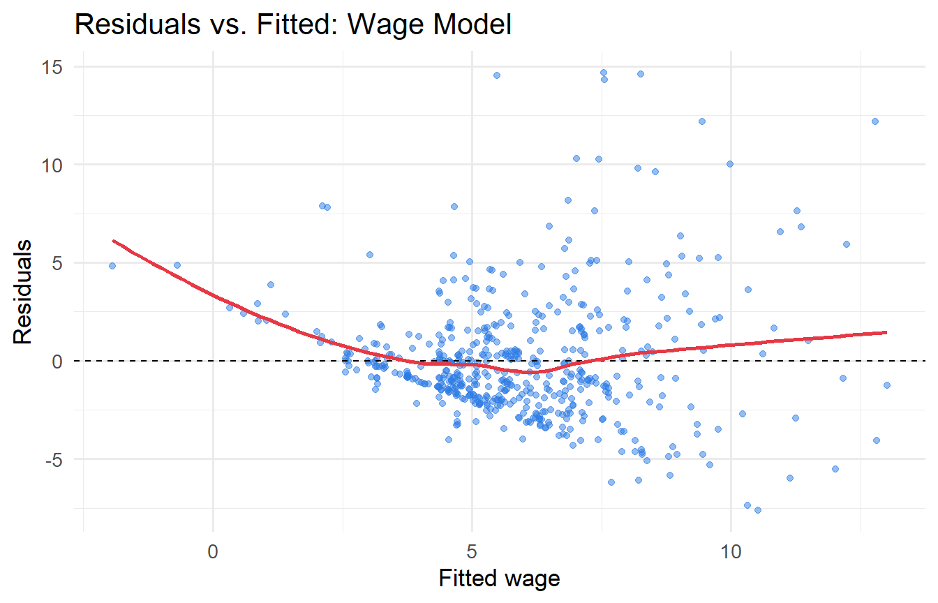
a. Plot the residuals against fitted values. Does the pattern suggest heteroskedasticity?
b. Conduct a Breusch-Pagan test. What do you conclude?
c. Report estimates with conventional and HC3 robust standard errors side by side. Which coefficients change meaningfully?
::: {.callout-tip collapse="true"}
## Solution
```{r}
#| label: ex9-1
fit_wage <- lm(wage ~ educ + exper + tenure, data = wage1)

# a) Residual plot
augment(fit_wage) |>
  ggplot(aes(.fitted, .resid)) +
  geom_point(alpha = 0.5, colour = "#2c7be5") +
  geom_hline(yintercept = 0, linetype = "dashed") +
  geom_smooth(method = "loess", se = FALSE, colour = "#e63946") +
  labs(x = "Fitted wage", y = "Residuals", title = "Residuals vs. Fitted: Wage Model")
# b) BP test
bptest(fit_wage)
# c) Comparison
fit_wage_r <- lm_robust(wage ~ educ + exper + tenure, data = wage1, se_type = "HC3")
modelsummary(
  list("OLS (conventional)" = fit_wage, "OLS (HC3 robust)" = fit_wage_r),
  stars = TRUE, gof_map = c("nobs", "r.squared")
)
```
The residual plot typically shows a fan shape — higher earners have more variable wages, a classic pattern. The BP test should be significant. Robust SEs are often larger for `educ`, which matters most for policy interpretation.
:::
**Tutorial 9.2**
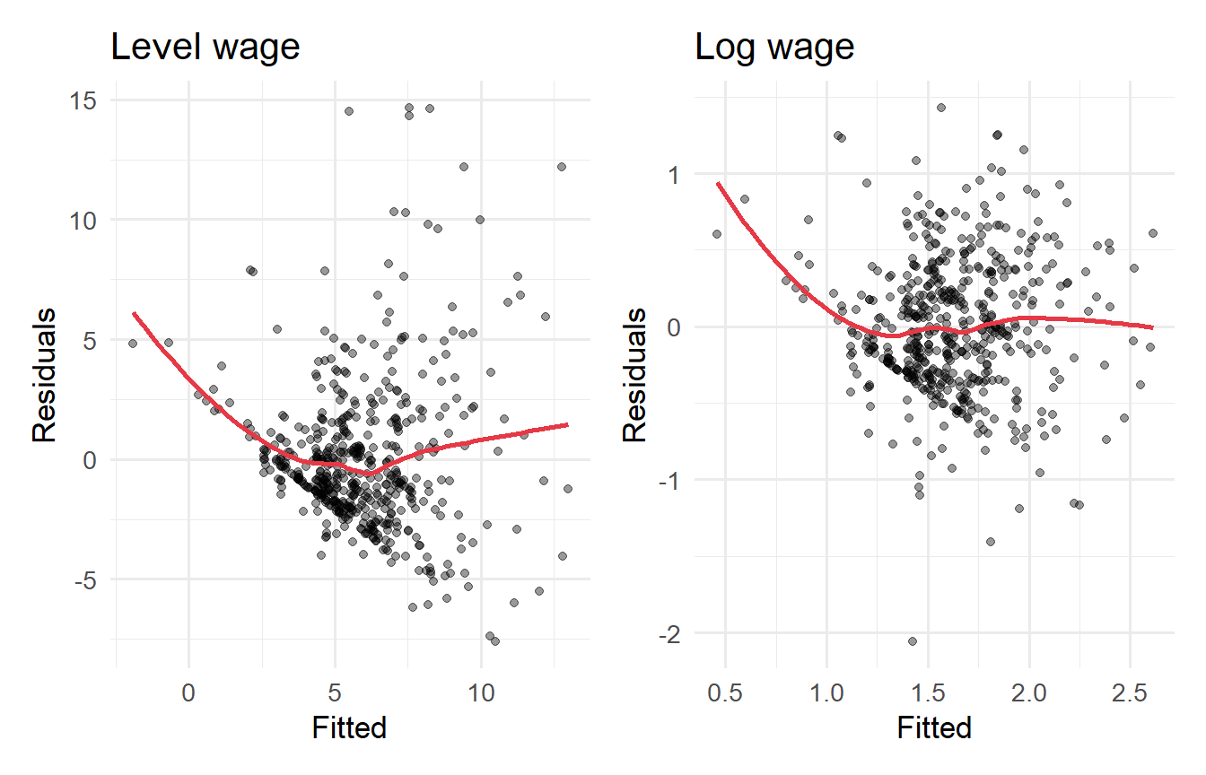
Show that the **log wage** specification reduces (but may not eliminate) heteroskedasticity. Regress `log(wage)` on `educ`, `exper`, and `tenure`, then apply the BP test and compare residual plots with the level-wage model.
::: {.callout-tip collapse="true"}
## Solution
```{r}
#| label: ex9-2
wage1 <- wage1 |> mutate(lwage = log(wage))
fit_lwage <- lm(lwage ~ educ + exper + tenure, data = wage1)

bptest(fit_wage)   # level model
bptest(fit_lwage) # log model
# Residual plots side by side
p1 <- augment(fit_wage) |>
  ggplot(aes(.fitted, .resid)) +
  geom_point(alpha = 0.4) + geom_smooth(method = "loess", se = FALSE, colour = "#e63946") +
  labs(title = "Level wage", x = "Fitted", y = "Residuals")

p2 <- augment(fit_lwage) |>
  ggplot(aes(.fitted, .resid)) +
  geom_point(alpha = 0.4) + geom_smooth(method = "loess", se = FALSE, colour = "#e63946") +
  labs(title = "Log wage", x = "Fitted", y = "Residuals")

library(patchwork)
p1 + p2
```
The log transformation substantially reduces heteroskedasticity. The BP test is often no longer significant (or much less so) for the log wage model. This is one reason why log specifications are so common in labour economics.
:::
**Tutorial 9.3**
Using `wooldridge::hprice1`, estimate the log-price model: `log(price) ~ log(sqrft) + bdrms + log(lotsize)`.
a. Apply the BP test. Is heteroskedasticity still present?
b. Compare OLS with HC3 robust standard errors for this log-log model.
c. Which approach do you prefer, and why? Consider both the BP test result and the change in inference.
::: {.callout-tip collapse="true"}
## Solution
```{r}
#| label: ex9-3
fit_log2 <- lm(log(price) ~ log(sqrft) + bdrms + log(lotsize), data = hprice1)

# a) BP test
bptest(fit_log2)
# b) Comparison
fit_log2_r <- lm_robust(log(price) ~ log(sqrft) + bdrms + log(lotsize),
                        data = hprice1, se_type = "HC3")

modelsummary(
  list("OLS (conventional)" = fit_log2, "OLS (HC3 robust)" = fit_log2_r),
  stars = TRUE, gof_map = c("nobs", "r.squared"),
  title = "Log-Price Model: Conventional vs. Robust SEs"
)
```
The BP test result for the log model is typically much weaker than for the level model. If heteroskedasticity is no longer significant, conventional SEs are adequate. However, as a matter of **robustness practice**, many applied economists report HC3 SEs regardless — the cost is minimal and the protection is real.
:::